Homework 5 Key

knitr::opts_chunk$set(comment = ">")
library(tidyverse)
library(ggrepel)
library(ggthemes)

Answer 2

Read in the data, clean up the names, and pivot it in a way so the first few rows look like this:

billboard <- read_csv("billboard_top100.csv") 
billboard_tidy <- billboard |> 
  pivot_longer(starts_with("wk"), 
               names_to = "week", 
               values_to = "rank", 
               values_drop_na = TRUE, 
               names_prefix = "wk", 
               names_transform = list(week = as.integer)) |> 
  janitor::clean_names() 
billboard_tidy

> # A tibble: 5,307 × 6
>    artist  track                   time   date_entered  week  rank
>    <chr>   <chr>                   <time> <date>       <int> <dbl>
>  1 2 Pac   Baby Don't Cry (Keep... 04:22  2000-02-26       1    87
>  2 2 Pac   Baby Don't Cry (Keep... 04:22  2000-02-26       2    82
>  3 2 Pac   Baby Don't Cry (Keep... 04:22  2000-02-26       3    72
>  4 2 Pac   Baby Don't Cry (Keep... 04:22  2000-02-26       4    77
>  5 2 Pac   Baby Don't Cry (Keep... 04:22  2000-02-26       5    87
>  6 2 Pac   Baby Don't Cry (Keep... 04:22  2000-02-26       6    94
>  7 2 Pac   Baby Don't Cry (Keep... 04:22  2000-02-26       7    99
>  8 2Ge+her The Hardest Part Of ... 03:15  2000-09-02       1    91
>  9 2Ge+her The Hardest Part Of ... 03:15  2000-09-02       2    87
> 10 2Ge+her The Hardest Part Of ... 03:15  2000-09-02       3    92
> # ℹ 5,297 more rows

Answer 3

Create a variable named date that corresponds to the week based on the date_entered.

billboard_tidy_date <- billboard_tidy |> 
  mutate(date = if_else(week == 1,
                       date_entered,
                       date_entered + weeks(x = week - 1)))
billboard_tidy_date

1

This if_else basically says, “if week is equal to 1 then assign the date_entered value to date. Otherwise, add the number of weeks minus 1 to the date_entered value (i.e. for the second week you would want to add 2 - 1 or 1 week to the date_entered value).

> # A tibble: 5,307 × 7
>    artist  track                   time   date_entered  week  rank date      
>    <chr>   <chr>                   <time> <date>       <int> <dbl> <date>    
>  1 2 Pac   Baby Don't Cry (Keep... 04:22  2000-02-26       1    87 2000-02-26
>  2 2 Pac   Baby Don't Cry (Keep... 04:22  2000-02-26       2    82 2000-03-04
>  3 2 Pac   Baby Don't Cry (Keep... 04:22  2000-02-26       3    72 2000-03-11
>  4 2 Pac   Baby Don't Cry (Keep... 04:22  2000-02-26       4    77 2000-03-18
>  5 2 Pac   Baby Don't Cry (Keep... 04:22  2000-02-26       5    87 2000-03-25
>  6 2 Pac   Baby Don't Cry (Keep... 04:22  2000-02-26       6    94 2000-04-01
>  7 2 Pac   Baby Don't Cry (Keep... 04:22  2000-02-26       7    99 2000-04-08
>  8 2Ge+her The Hardest Part Of ... 03:15  2000-09-02       1    91 2000-09-02
>  9 2Ge+her The Hardest Part Of ... 03:15  2000-09-02       2    87 2000-09-09
> 10 2Ge+her The Hardest Part Of ... 03:15  2000-09-02       3    92 2000-09-16
> # ℹ 5,297 more rows

Answer 4

Create a dataset of the song(s) with the most weeks in the top 3 by month of 2000.

billboard_top3_month <- billboard_tidy_date |> 
  mutate(month = month(date),
         year = year(date),
         top3 = if_else(rank <= 3 & year == 2000, 1, 0)) |>
  mutate(peak_weeks = sum(top3),
         .by = c(month, artist, track)) |>
  slice_max(peak_weeks,
            by = month) |>
  distinct(month, artist, track, peak_weeks) |>
  arrange(month)
billboard_top3_month

1

We need to be able to filter rows by month so we need to create a month variable from our date variable.

2

This dataset is about the 2000 top 100 but many of these songs charted before or after that year. Therefore, we will need a variable for year as well so we make sure we’re finding the songs that charted in the months of 2000.

3

To create our top3 indicator we provide the two conditions that the rank for that observation is less than or equal to 3 AND the year is 2000. If so, top3 will be assigned a value of 1 and if not it will get a value of 0.

4

To filter for the most weeks in the top 3 we need to count how many weeks a song was in the top 3, grouped by month, song, and artist.

5

Then, by month we can slice the song(s) with the most weeks in the top 3.

6

Now we just want the name of the artist, song, the month they were charting in the top 3 for the most weeks, and the number of weeks

7

To see this in chronological order we want to arrange by the month

> # A tibble: 19 × 4
>    month artist              track                   peak_weeks
>    <dbl> <chr>               <chr>                        <dbl>
>  1     1 Aguilera, Christina What A Girl Wants                3
>  2     2 Savage Garden       I Knew I Loved You               4
>  3     3 Lonestar            Amazed                           4
>  4     4 Hill, Faith         Breathe                          5
>  5     4 Santana             Maria, Maria                     5
>  6     5 Hill, Faith         Breathe                          4
>  7     5 Santana             Maria, Maria                     4
>  8     6 Aaliyah             Try Again                        2
>  9     6 Anthony, Marc       You Sang To Me                   2
> 10     6 Hill, Faith         Breathe                          2
> 11     6 Santana             Maria, Maria                     2
> 12     6 Vertical Horizon    Everything You Want              2
> 13     7 Aaliyah             Try Again                        4
> 14     8 Sisqo               Incomplete                       4
> 15     8 matchbox twenty     Bent                             4
> 16     9 Janet               Doesn't Really Matte...          5
> 17    10 Madonna             Music                            4
> 18    11 Creed               With Arms Wide Open              4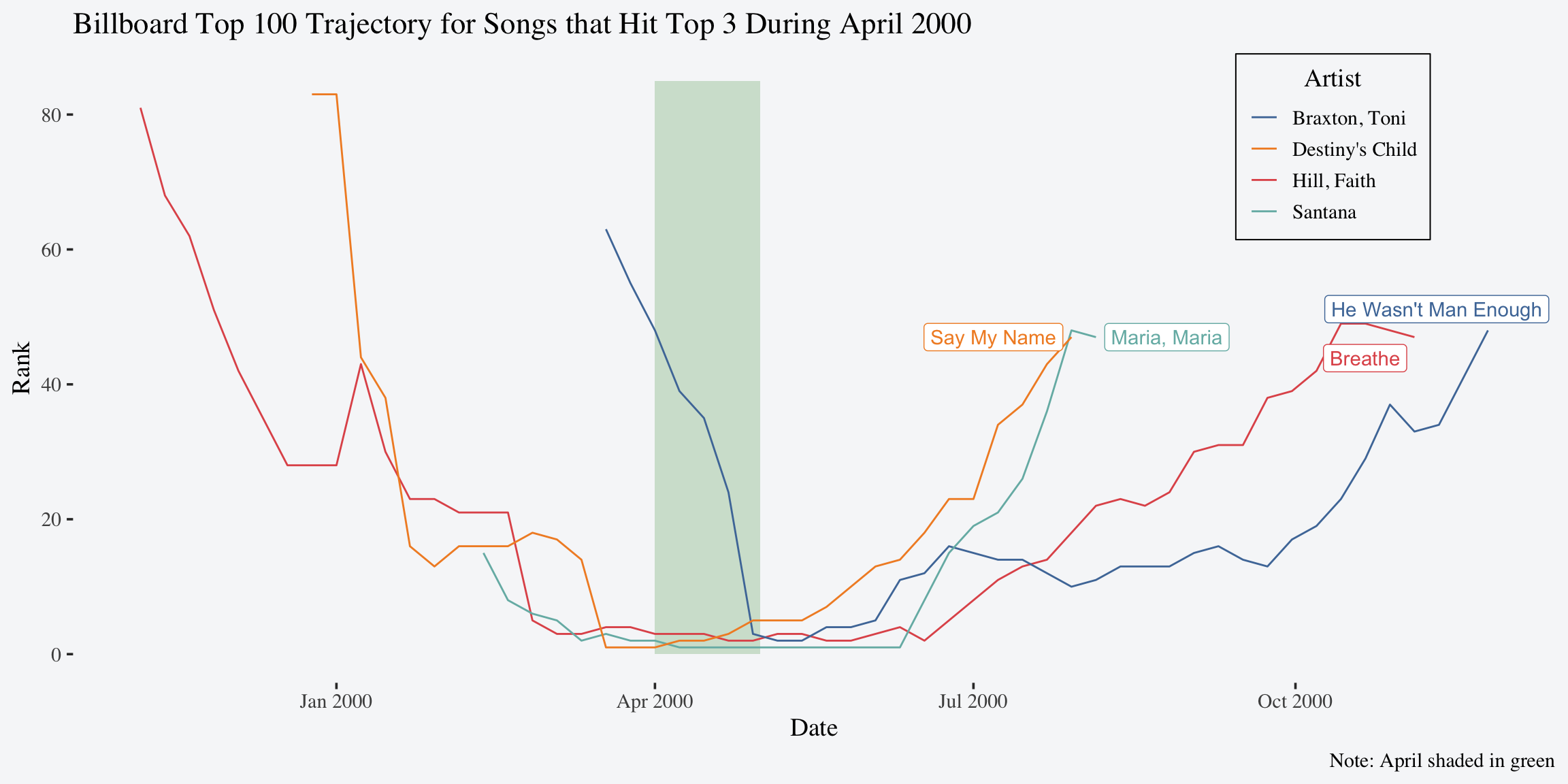
> 19    12 Destiny's Child     Independent Women Pa...          5

Answer 5

Pick one month of 2000 and visualize the entire charting trajectory of the songs that spent at least 1 week in the top 3 during that month.

billboard_top3_month_viz <- billboard_tidy_date |> 
  mutate(month = month(date),
         year = year(date),
         top3 = if_else(rank <= 3 & year == 2000, 1, 0)) |> 
  mutate(month_peak = ifelse(top3 == 1, month, NA),
         .by = c(month, artist, track)) |> 
  filter(any(month_peak == 4),
         .by = c(track, artist)) 

ggplot(billboard_top3_month_viz, aes(date, rank, group = track, color = artist)) + 
  annotate(geom = "rect", xmin = ymd("2000-04-01"), xmax = ymd("2000-05-01"), ymin = 0, ymax = 85,
           fill = "#59a14f", alpha = 0.25) +
  geom_line(show.legend = TRUE) +
  geom_label_repel(data = billboard_top3_month_viz |> slice_max(date, by = track),
                   aes(label = track), 
                   show.legend = FALSE) +
  scale_color_manual("Artist", values = c("#4e79a7","#f28e2c","#e15759","#76b7b2")) +
  labs(title = "Billboard Top 100 Trajectory for Songs that Hit Top 3 During April 2000", 
       x = "Date", 
       y = "Rank", 
       caption = "Note: April shaded in green") + 
  theme_tufte(base_size = 14) + 
  theme(legend.position = c(0.85, 0.85),
        legend.title.align = 0.5,
        legend.box.background = element_rect(colour = "black", fill = "#f6f7f9"),
        plot.background = element_rect(fill = "#f6f7f9", color = "#f6f7f9"))

1

In order to visualize the entire trajectory, we need to have a variable that indicates when a song was charting in the top 3

2

This allows us to filter by each song whether any of the weeks charted in the top 3 for the month we’re interested in. Without these two steps we could only filter for the weeks in which they were charting and therefore couldn’t plot their entire ranking trajectory.

3

Shading the region for April for reference.

4

Want the legend for the line to appear.

5

Need to use a subset of the data otherwise each row will try to plot a label; I picked the last charting date for each song.

6

Wanted to remove the legend for the label (a lower-case “a”).

7

Specifying the colors I want to use for the 4 different lines.

8

Moving the legend to maximize plotting space.

9

Centering the legend title in the legend box.

10

Putting a black border around the legend.

11

Changing the plot color to the same color as the website.