Below is one possible way you may have organized your folder for this class into a project/series of projects. Note: for whichever folder you set as a project(s) you will have a .Rproj file which maintains specific project settings. That project folder is your default working directory when you’re doing any work within this folder (including within subfolders). Individual .qmd files will have a working directory of the specific folder they are in when they are rendered. Keep this in mind when trying to run code from a source document saved in a folder separate from its associated project folder.
If you want to simultaneously create and call an object to see what it looks like you can put parentheses around the entire assignment and it will be created and called in one step!
rnorm takes a number of observations (n) and a specified mean (mean) and standard deviation (sd). It returns n number of random deviates from the normal distribution with the specified mean and standard deviation.
n is required but mean and sd are optional. If they are not specified they default to 0 and 1 respectively.
When writing a conditional argument you always include the object you’re evaluating. This also allows you to make comparisons of x to conditional statements of different vectors of the same length. See example below.
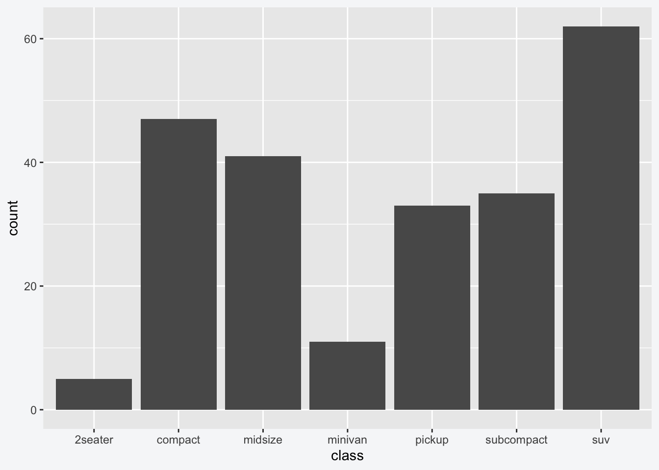
The second plot is saved because the default for ggsave() when not explicitly given a plot object as the second argument is to save the last plot displayed.
The plot image mpg-plot.png should have been added to your current project folder. Note: If your project is at the course level and you’re running this interactively, it will be saved in the overall course folder. When you render the file for homework3.qmd it will be saved in whichever folder that file is saved (i.e. the project folder is always the working durectory when you’re running code interactively in an R session. Each rendered file has a working directory of whichever folder they are saved to).
One of my favorite keyboard shortcuts is multi-cursor editing which is demonstrated in this subsection. If you use Ctrl + Alt_left + Mouse_left you can create new cursors wherever you click your mouse. This then allows you to type something once and have it repeated wherever the cursors are.
Answer 5
y <-tibble(a =seq(1, 10, 2), b =c("apple", "banana", "strawberry", "peach", "mango"), c =c(rep(TRUE, 3), rep(FALSE, 2)))y
> # A tibble: 5 × 3
>       a b          c
>   <dbl> <chr>      <lgl>
> 1     1 apple      TRUE
> 2     3 banana     TRUE
> 3     5 strawberry TRUE
> 4     7 peach      FALSE
> 5     9 mango      FALSE
seq creates a sequence of numbers from the first argument from to the second argument to by increments of the third argument by.
rep repeats the first argument x by the second argument which can be the integer number of times, length.out (length of final vector), or each (how many times each element of x should be repeated).
y[c(2, 5), 2]
> # A tibble: 2 × 1
>   b
>   <chr>
> 1 banana
> 2 mango
y$c
> [1] TRUE TRUE TRUE FALSE FALSE
y[3:5, ] prints out the 3rd, 4th, and 5th rows and : is a shortcut for giving a sequence from the first number (on the left) to the second number (on the right) in increments of 1 or -1.