Data Wrangling in R

CSSCR Workshop

31 October 2024

Victoria Sass

Roadmap

• Importing and Exporting Data
• Manipulating and Summarizing Data
• Merging Data
• Tidying and Reshaping Data

Importing and Exporting Data

Data Packages

R has a big user base. If you are working with a popular data source, it will often have a devoted R package on CRAN or Github.

Examples:

• WDI: World Development Indicators (World Bank)
• tidycensus: Census and American Community Survey
• quantmod: financial data from Yahoo, FRED, Google
• gssr: The General Social Survey Cumulative Data (1972-2021)
• psidR: Panel Study of Income Dynamics (basic & public datasets)

If you have an actual data file, you’ll have to import it yourself…

Delimited Text Files

Besides a package, it’s easiest when data is stored in a text file. The most commonly encountered delimited file is a .csv.

A comma-separated values (.csv) file looks like the following:

"Subject","Depression","Sex","Week","HamD","Imipramine"
101,"Non-endogenous","Second",0,26,NA
101,"Non-endogenous","Second",1,22,NA
101,"Non-endogenous","Second",2,18,4.04305
101,"Non-endogenous","Second",3,7,3.93183
101,"Non-endogenous","Second",4,4,4.33073
101,"Non-endogenous","Second",5,3,4.36945
103,"Non-endogenous","First",0,33,NA
103,"Non-endogenous","First",1,24,NA
103,"Non-endogenous","First",2,15,2.77259

readr

R has some built-in functions for importing data, such as read.table() and read.csv().

The readr package provides similar functions, like read_csv(), that have slightly better features:

• Faster!
• Better defaults (e.g. doesn’t automatically convert characters to factors)
• A bit smarter about dates and times
• Loading progress bars for large files

readr is one of the core tidyverse packages so loading tidyverse will load it too:

library(tidyverse)

Alternatively, you can just load readr like so:

library(readr)

readr Importing Example

Let’s import some data about song ranks on the Billboard Hot 100 in 2000:

billboard_2000_raw <- read_csv(file = "data/billboard.csv")

How do we know it loaded?

Let’s look at it!

glimpse(billboard_2000_raw)

Rows: 317
Columns: 81
$ year         <dbl> 2000, 2000, 2000, 2000, 2000, 2000, 2000, 2000, 2000, 200…
$ artist       <chr> "2 Pac", "2Ge+her", "3 Doors Down", "3 Doors Down", "504 …
$ track        <chr> "Baby Don't Cry (Keep...", "The Hardest Part Of ...", "Kr…
$ time         <time> 04:22:00, 03:15:00, 03:53:00, 04:24:00, 03:35:00, 03:24:…
$ date.entered <date> 2000-02-26, 2000-09-02, 2000-04-08, 2000-10-21, 2000-04-…
$ wk1          <dbl> 87, 91, 81, 76, 57, 51, 97, 84, 59, 76, 84, 57, 50, 71, 7…
$ wk2          <dbl> 82, 87, 70, 76, 34, 39, 97, 62, 53, 76, 84, 47, 39, 51, 6…
$ wk3          <dbl> 72, 92, 68, 72, 25, 34, 96, 51, 38, 74, 75, 45, 30, 28, 5…
$ wk4          <dbl> 77, NA, 67, 69, 17, 26, 95, 41, 28, 69, 73, 29, 28, 18, 4…
$ wk5          <dbl> 87, NA, 66, 67, 17, 26, 100, 38, 21, 68, 73, 23, 21, 13, …
$ wk6          <dbl> 94, NA, 57, 65, 31, 19, NA, 35, 18, 67, 69, 18, 19, 13, 3…
$ wk7          <dbl> 99, NA, 54, 55, 36, 2, NA, 35, 16, 61, 68, 11, 20, 11, 34…
$ wk8          <dbl> NA, NA, 53, 59, 49, 2, NA, 38, 14, 58, 65, 9, 17, 1, 29, …
$ wk9          <dbl> NA, NA, 51, 62, 53, 3, NA, 38, 12, 57, 73, 9, 17, 1, 27, …
$ wk10         <dbl> NA, NA, 51, 61, 57, 6, NA, 36, 10, 59, 83, 11, 17, 2, 30,…
$ wk11         <dbl> NA, NA, 51, 61, 64, 7, NA, 37, 9, 66, 92, 1, 17, 2, 36, N…
$ wk12         <dbl> NA, NA, 51, 59, 70, 22, NA, 37, 8, 68, NA, 1, 3, 3, 37, N…
$ wk13         <dbl> NA, NA, 47, 61, 75, 29, NA, 38, 6, 61, NA, 1, 3, 3, 39, N…
$ wk14         <dbl> NA, NA, 44, 66, 76, 36, NA, 49, 1, 67, NA, 1, 7, 4, 49, N…
$ wk15         <dbl> NA, NA, 38, 72, 78, 47, NA, 61, 2, 59, NA, 4, 10, 12, 57,…
$ wk16         <dbl> NA, NA, 28, 76, 85, 67, NA, 63, 2, 63, NA, 8, 17, 11, 63,…
$ wk17         <dbl> NA, NA, 22, 75, 92, 66, NA, 62, 2, 67, NA, 12, 25, 13, 65…
$ wk18         <dbl> NA, NA, 18, 67, 96, 84, NA, 67, 2, 71, NA, 22, 29, 15, 68…
$ wk19         <dbl> NA, NA, 18, 73, NA, 93, NA, 83, 3, 79, NA, 23, 29, 18, 79…
$ wk20         <dbl> NA, NA, 14, 70, NA, 94, NA, 86, 4, 89, NA, 43, 40, 20, 86…
$ wk21         <dbl> NA, NA, 12, NA, NA, NA, NA, NA, 5, NA, NA, 44, 43, 30, NA…
$ wk22         <dbl> NA, NA, 7, NA, NA, NA, NA, NA, 5, NA, NA, NA, 50, 40, NA,…
$ wk23         <dbl> NA, NA, 6, NA, NA, NA, NA, NA, 6, NA, NA, NA, NA, 39, NA,…
$ wk24         <dbl> NA, NA, 6, NA, NA, NA, NA, NA, 9, NA, NA, NA, NA, 44, NA,…
$ wk25         <dbl> NA, NA, 6, NA, NA, NA, NA, NA, 13, NA, NA, NA, NA, NA, NA…
$ wk26         <dbl> NA, NA, 5, NA, NA, NA, NA, NA, 14, NA, NA, NA, NA, NA, NA…
$ wk27         <dbl> NA, NA, 5, NA, NA, NA, NA, NA, 16, NA, NA, NA, NA, NA, NA…
$ wk28         <dbl> NA, NA, 4, NA, NA, NA, NA, NA, 23, NA, NA, NA, NA, NA, NA…
$ wk29         <dbl> NA, NA, 4, NA, NA, NA, NA, NA, 22, NA, NA, NA, NA, NA, NA…
$ wk30         <dbl> NA, NA, 4, NA, NA, NA, NA, NA, 33, NA, NA, NA, NA, NA, NA…
$ wk31         <dbl> NA, NA, 4, NA, NA, NA, NA, NA, 36, NA, NA, NA, NA, NA, NA…
$ wk32         <dbl> NA, NA, 3, NA, NA, NA, NA, NA, 43, NA, NA, NA, NA, NA, NA…
$ wk33         <dbl> NA, NA, 3, NA, NA, NA, NA, NA, NA, NA, NA, NA, NA, NA, NA…
$ wk34         <dbl> NA, NA, 3, NA, NA, NA, NA, NA, NA, NA, NA, NA, NA, NA, NA…
$ wk35         <dbl> NA, NA, 4, NA, NA, NA, NA, NA, NA, NA, NA, NA, NA, NA, NA…
$ wk36         <dbl> NA, NA, 5, NA, NA, NA, NA, NA, NA, NA, NA, NA, NA, NA, NA…
$ wk37         <dbl> NA, NA, 5, NA, NA, NA, NA, NA, NA, NA, NA, NA, NA, NA, NA…
$ wk38         <dbl> NA, NA, 9, NA, NA, NA, NA, NA, NA, NA, NA, NA, NA, NA, NA…
$ wk39         <dbl> NA, NA, 9, NA, NA, NA, NA, NA, NA, NA, NA, NA, NA, NA, NA…
$ wk40         <dbl> NA, NA, 15, NA, NA, NA, NA, NA, NA, NA, NA, NA, NA, NA, N…
$ wk41         <dbl> NA, NA, 14, NA, NA, NA, NA, NA, NA, NA, NA, NA, NA, NA, N…
$ wk42         <dbl> NA, NA, 13, NA, NA, NA, NA, NA, NA, NA, NA, NA, NA, NA, N…
$ wk43         <dbl> NA, NA, 14, NA, NA, NA, NA, NA, NA, NA, NA, NA, NA, NA, N…
$ wk44         <dbl> NA, NA, 16, NA, NA, NA, NA, NA, NA, NA, NA, NA, NA, NA, N…
$ wk45         <dbl> NA, NA, 17, NA, NA, NA, NA, NA, NA, NA, NA, NA, NA, NA, N…
$ wk46         <dbl> NA, NA, 21, NA, NA, NA, NA, NA, NA, NA, NA, NA, NA, NA, N…
$ wk47         <dbl> NA, NA, 22, NA, NA, NA, NA, NA, NA, NA, NA, NA, NA, NA, N…
$ wk48         <dbl> NA, NA, 24, NA, NA, NA, NA, NA, NA, NA, NA, NA, NA, NA, N…
$ wk49         <dbl> NA, NA, 28, NA, NA, NA, NA, NA, NA, NA, NA, NA, NA, NA, N…
$ wk50         <dbl> NA, NA, 33, NA, NA, NA, NA, NA, NA, NA, NA, NA, NA, NA, N…
$ wk51         <dbl> NA, NA, 42, NA, NA, NA, NA, NA, NA, NA, NA, NA, NA, NA, N…
$ wk52         <dbl> NA, NA, 42, NA, NA, NA, NA, NA, NA, NA, NA, NA, NA, NA, N…
$ wk53         <dbl> NA, NA, 49, NA, NA, NA, NA, NA, NA, NA, NA, NA, NA, NA, N…
$ wk54         <dbl> NA, NA, NA, NA, NA, NA, NA, NA, NA, NA, NA, NA, NA, NA, N…
$ wk55         <dbl> NA, NA, NA, NA, NA, NA, NA, NA, NA, NA, NA, NA, NA, NA, N…
$ wk56         <dbl> NA, NA, NA, NA, NA, NA, NA, NA, NA, NA, NA, NA, NA, NA, N…
$ wk57         <dbl> NA, NA, NA, NA, NA, NA, NA, NA, NA, NA, NA, NA, NA, NA, N…
$ wk58         <dbl> NA, NA, NA, NA, NA, NA, NA, NA, NA, NA, NA, NA, NA, NA, N…
$ wk59         <dbl> NA, NA, NA, NA, NA, NA, NA, NA, NA, NA, NA, NA, NA, NA, N…
$ wk60         <dbl> NA, NA, NA, NA, NA, NA, NA, NA, NA, NA, NA, NA, NA, NA, N…
$ wk61         <dbl> NA, NA, NA, NA, NA, NA, NA, NA, NA, NA, NA, NA, NA, NA, N…
$ wk62         <dbl> NA, NA, NA, NA, NA, NA, NA, NA, NA, NA, NA, NA, NA, NA, N…
$ wk63         <dbl> NA, NA, NA, NA, NA, NA, NA, NA, NA, NA, NA, NA, NA, NA, N…
$ wk64         <dbl> NA, NA, NA, NA, NA, NA, NA, NA, NA, NA, NA, NA, NA, NA, N…
$ wk65         <dbl> NA, NA, NA, NA, NA, NA, NA, NA, NA, NA, NA, NA, NA, NA, N…
$ wk66         <lgl> NA, NA, NA, NA, NA, NA, NA, NA, NA, NA, NA, NA, NA, NA, N…
$ wk67         <lgl> NA, NA, NA, NA, NA, NA, NA, NA, NA, NA, NA, NA, NA, NA, N…
$ wk68         <lgl> NA, NA, NA, NA, NA, NA, NA, NA, NA, NA, NA, NA, NA, NA, N…
$ wk69         <lgl> NA, NA, NA, NA, NA, NA, NA, NA, NA, NA, NA, NA, NA, NA, N…
$ wk70         <lgl> NA, NA, NA, NA, NA, NA, NA, NA, NA, NA, NA, NA, NA, NA, N…
$ wk71         <lgl> NA, NA, NA, NA, NA, NA, NA, NA, NA, NA, NA, NA, NA, NA, N…
$ wk72         <lgl> NA, NA, NA, NA, NA, NA, NA, NA, NA, NA, NA, NA, NA, NA, N…
$ wk73         <lgl> NA, NA, NA, NA, NA, NA, NA, NA, NA, NA, NA, NA, NA, NA, N…
$ wk74         <lgl> NA, NA, NA, NA, NA, NA, NA, NA, NA, NA, NA, NA, NA, NA, N…
$ wk75         <lgl> NA, NA, NA, NA, NA, NA, NA, NA, NA, NA, NA, NA, NA, NA, N…
$ wk76         <lgl> NA, NA, NA, NA, NA, NA, NA, NA, NA, NA, NA, NA, NA, NA, N…

Alternate Solution

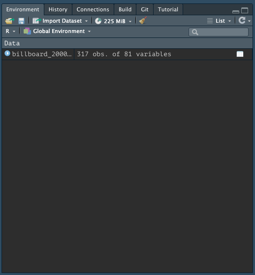
When you import data from an external file you’ll also see it in the Global Environment tab in the upper-right pane of RStudio:

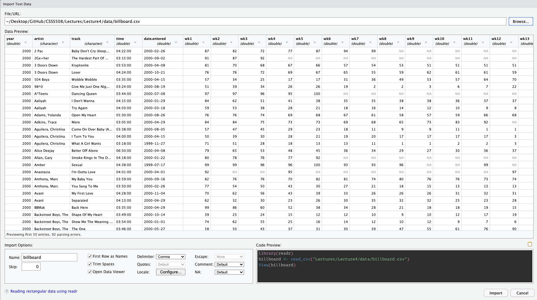
You can also import the data manually!

In the upper right-hand pane of RStudio (make sure you’re in the Environment tab), select:

Import Dataset > From Text (readr) and browse to the file on your computer¹.

Once you’ve imported the data, you can copy/paste the import code from the console into your file!!

This makes the process reproducible!

1. Ideally you’ve saved it in your project folder!

Manual Data Import

Specifying NAs

Sometimes a particular dataset or file read from a different software will code NAs differently than R. If that’s the case, you can add additional specifications to read_csv for what to read in as NA.

billboard_2000_raw <- read_csv(file = "data/billboard.csv", 
                               na = c("N/A", "999"))

Skipping lines

Depending on how the data were input, there may be several lines that precede the beginning of the data table you’re interested in importing. You can skip these lines of metadata with the skip argument:

billboard_2000_raw <- read_csv(file = "data/billboard.csv", 
                               skip = 1)

Variable names

read_csv will automatically take the first row as column names. If you want to rename them you can save yourself some time recoding later on if you specify your preferred variable names upfront with the col_names argument.

It takes a character vector to be used as column names (in their order of appearance).

billboard_renamed <- read_csv(file = "data/billboard.csv",
                              col_names = c("year", "artist", "track", "time", "date_entered", 
                                            paste("wk", 1:76, sep = "_")))

billboard_renamed |>  names() |> head(10)

1

First few entries: “wk_1” “wk_2” “wk_3”

2

names returns the column names.

 [1] "year"         "artist"       "track"        "time"         "date_entered"
 [6] "wk_1"         "wk_2"         "wk_3"         "wk_4"         "wk_5"        

If you don’t have any variable names you can specify that instead.

billboard_2000_raw <- read_csv(file = "data/billboard.csv", 
                               col_names = FALSE) 

Snake Case

If you simply want to change your variables to snake case (all lower case; words separated by _), you can use the function clean_names() from the janitor package which replaces other punctuation separators with _.

# Download package first
# install.packages("janitor")

# Create new object for renamed data
billboard_renamed <- billboard_2000_raw |> 
  janitor::clean_names(numerals = "right")

billboard_renamed |>  names() |> head(10)

3

Run in the console first.

4

You can call a function without loading its package by specifying its package name followed by :: before it;
The numerals argument specifies if you additionally want to put a separator before a number.

 [1] "year"         "artist"       "track"        "time"         "date_entered"
 [6] "wk_1"         "wk_2"         "wk_3"         "wk_4"         "wk_5"        

Other Data File Types with readr

The other functions in readr employ a similar approach to read_csv so the trick is just knowing which to use for what data type.

• read_csv2 is separated by semicolons (instead of commas)
• read_tsv is separated by tabs
• read_delim guesses the delimiter
• read_fwf reads in fixed-width-files
• read_table is a variation of fwf where columns are separated by white space
• read_log reads in Apache-style log files

Other Packages to Read in Data

There are a range of other ways, besides delimited files, that data are stored.

The following packages are part of the extended tidyverse and therefore operate with similar syntax and logic as readr.

Other Packages to Read in Data

There are a range of other ways, besides delimited files, that data are stored.

The following packages are part of the extended tidyverse and therefore operate with similar syntax and logic as readr.

• For Excel files (.xls or .xlsx), use package readxl¹

Note: For Excel files and Googlesheets You won’t keep text formatting, color, comments, or merged cells. See the openxlsx package for those capabilities. Also, tidyxl can help import non-tabular data from Excel.

1. Functions have additional arguments to read in specific sheets or a range of cells.

Other Packages to Read in Data

There are a range of other ways, besides delimited files, that data are stored.

The following packages are part of the extended tidyverse and therefore operate with similar syntax and logic as readr.

• For Excel files (.xls or .xlsx), use package readxl¹
• For Google Docs Spreadsheets, use package googlesheets4²

Note: For Excel files and Googlesheets You won’t keep text formatting, color, comments, or merged cells. See the openxlsx package for those capabilities. Also, tidyxl can help import non-tabular data from Excel.

1. Functions have additional arguments to read in specific sheets or a range of cells.

2. Very similar to readxl with some slight variations you can read about here.

Other Packages to Read in Data

There are a range of other ways, besides delimited files, that data are stored.

The following packages are part of the extended tidyverse and therefore operate with similar syntax and logic as readr.

• For Excel files (.xls or .xlsx), use package readxl¹
• For Google Docs Spreadsheets, use package googlesheets4²
• For Stata, SPSS, and SAS files, use package haven³

Note: For Excel files and Googlesheets You won’t keep text formatting, color, comments, or merged cells. See the openxlsx package for those capabilities. Also, tidyxl can help import non-tabular data from Excel.

1. Functions have additional arguments to read in specific sheets or a range of cells.

2. Very similar to readxl with some slight variations you can read about here.

3. SAS, SPSS, and Stata have so-called “labelled” vectors for which haven provides a class to represent in R. Alternatively, you can get rid of them with these functions.

How does readr parse different data types?

For each column in a data frame, readr functions pull the first 1000 rows and checks:

flowchart LR
    id1((Variable))==>A(["1. Does it contain only F, T, FALSE, TRUE, or NA (ignoring case)?"])==>id2{{Logical}}
    id1((Variable))==>B(["2. Does it contain only numbers (e.g., 1, -4.5, 5e6, Inf?)"])==>id3{{Number}}
    id1((Variable))==>C(["3. Does it match the ISO8601 standard?"])==>id4{{Date/Date-time}}
    id1((Variable))==>D(["4. None of the above"])==>id5{{String}}
    style id1 fill:#4B2E83,color:#B7A57A,stroke:#B7A57A
    style id2 fill:#B7A57A,color:#4B2E83,stroke:#4B2E83
    style id3 fill:#B7A57A,color:#4B2E83,stroke:#4B2E83
    style id4 fill:#B7A57A,color:#4B2E83,stroke:#4B2E83
    style id5 fill:#B7A57A,color:#4B2E83,stroke:#4B2E83
    style A fill:#FFFFFF,color:#000000,stroke:#000000
    style B fill:#FFFFFF,color:#000000,stroke:#000000
    style C fill:#FFFFFF,color:#000000,stroke:#000000
    style D fill:#FFFFFF,color:#000000,stroke:#000000

How does readr parse different data types?

For each column in a data frame, readr functions pull the first 1000 rows and checks:

flowchart LR
    id1((Variable))==>A(["1. Does it contain only F, T, FALSE, TRUE, or NA (ignoring case)?"])==>id2{{Logical}}
    id1((Variable))==>B(["2. Does it contain only numbers (e.g., 1, -4.5, 5e6, Inf?)"])==>id3{{Number}}
    id1((Variable))==>C(["3. Does it match the ISO8601 standard?"])==>id4{{Date/Date-time}}
    id1((Variable))==>D(["4. None of the above"])==>id5{{String}}
    style id1 fill:#4B2E83,color:#B7A57A,stroke:#B7A57A
    style id2 fill:#4B2E83,color:#B7A57A,stroke:#B7A57A
    style id3 fill:#B7A57A,color:#4B2E83,stroke:#4B2E83
    style id4 fill:#B7A57A,color:#4B2E83,stroke:#4B2E83
    style id5 fill:#B7A57A,color:#4B2E83,stroke:#4B2E83
    style A fill:#B7A57A,color:#000000,stroke:#000000
    style B fill:#FFFFFF,color:#000000,stroke:#000000
    style C fill:#FFFFFF,color:#000000,stroke:#000000
    style D fill:#FFFFFF,color:#000000,stroke:#000000

How does readr parse different data types?

For each column in a data frame, readr functions pull the first 1000 rows and checks:

flowchart LR
    id1((Variable))==>A(["1. Does it contain only F, T, FALSE, TRUE, or NA (ignoring case)?"])==>id2{{Logical}}
    id1((Variable))==>B(["2. Does it contain only numbers (e.g., 1, -4.5, 5e6, Inf?)"])==>id3{{Number}}
    id1((Variable))==>C(["3. Does it match the ISO8601 standard?"])==>id4{{Date/Date-time}}
    id1((Variable))==>D(["4. None of the above"])==>id5{{String}}
    style id1 fill:#4B2E83,color:#B7A57A,stroke:#B7A57A
    style id2 fill:#B7A57A,color:#4B2E83,stroke:#4B2E83
    style id3 fill:#4B2E83,color:#B7A57A,stroke:#B7A57A
    style id4 fill:#B7A57A,color:#4B2E83,stroke:#4B2E83
    style id5 fill:#B7A57A,color:#4B2E83,stroke:#4B2E83
    style A fill:#FFFFFF,color:#000000,stroke:#000000
    style B fill:#B7A57A,color:#000000,stroke:#000000
    style C fill:#FFFFFF,color:#000000,stroke:#000000
    style D fill:#FFFFFF,color:#000000,stroke:#000000

How does readr parse different data types?

For each column in a data frame, readr functions pull the first 1000 rows and checks:

flowchart LR
    id1((Variable))==>A(["1. Does it contain only F, T, FALSE, TRUE, or NA (ignoring case)?"])==>id2{{Logical}}
    id1((Variable))==>B(["2. Does it contain only numbers (e.g., 1, -4.5, 5e6, Inf?)"])==>id3{{Number}}
    id1((Variable))==>C(["3. Does it match the ISO8601 standard?"])==>id4{{Date/Date-time}}
    id1((Variable))==>D(["4. None of the above"])==>id5{{String}}
    style id1 fill:#4B2E83,color:#B7A57A,stroke:#B7A57A
    style id2 fill:#B7A57A,color:#4B2E83,stroke:#4B2E83
    style id3 fill:#B7A57A,color:#4B2E83,stroke:#4B2E83
    style id4 fill:#4B2E83,color:#B7A57A,stroke:#B7A57A
    style id5 fill:#B7A57A,color:#4B2E83,stroke:#4B2E83
    style A fill:#FFFFFF,color:#000000,stroke:#000000
    style B fill:#FFFFFF,color:#000000,stroke:#000000
    style C fill:#B7A57A,color:#000000,stroke:#000000
    style D fill:#FFFFFF,color:#000000,stroke:#000000

How does readr parse different data types?

For each column in a data frame, readr functions pull the first 1000 rows and checks:

flowchart LR
    id1((Variable))==>A(["1. Does it contain only F, T, FALSE, TRUE, or NA (ignoring case)?"])==>id2{{Logical}}
    id1((Variable))==>B(["2. Does it contain only numbers (e.g., 1, -4.5, 5e6, Inf?)"])==>id3{{Number}}
    id1((Variable))==>C(["3. Does it match the ISO8601 standard?"])==>id4{{Date/Date-time}}
    id1((Variable))==>D(["4. None of the above"])==>id5{{String}}
    style id1 fill:#4B2E83,color:#B7A57A,stroke:#B7A57A
    style id2 fill:#B7A57A,color:#4B2E83,stroke:#4B2E83
    style id3 fill:#B7A57A,color:#4B2E83,stroke:#4B2E83
    style id4 fill:#B7A57A,color:#4B2E83,stroke:#4B2E83
    style id5 fill:#4B2E83,color:#B7A57A,stroke:#B7A57A
    style A fill:#FFFFFF,color:#000000,stroke:#000000
    style B fill:#FFFFFF,color:#000000,stroke:#000000
    style C fill:#FFFFFF,color:#000000,stroke:#000000
    style D fill:#B7A57A,color:#000000,stroke:#000000

Most Common Issue with Reading in Data

The most common problem that occurs when reading in data is having mixed data. Most often, given the heuristic provided in the last slide, R will parse a variable as a character string to preserve whatever it contains.

Let’s actually look at how the billboard data was read in:

glimpse(billboard_2000_raw) 

Rows: 317
Columns: 81
$ year         <dbl> 2000, 2000, 2000, 2000, 2000, 2000, 2000, 2000, 2000, 200…
$ artist       <chr> "2 Pac", "2Ge+her", "3 Doors Down", "3 Doors Down", "504 …
$ track        <chr> "Baby Don't Cry (Keep...", "The Hardest Part Of ...", "Kr…
$ time         <time> 04:22:00, 03:15:00, 03:53:00, 04:24:00, 03:35:00, 03:24:…
$ date.entered <date> 2000-02-26, 2000-09-02, 2000-04-08, 2000-10-21, 2000-04-…
$ wk1          <dbl> 87, 91, 81, 76, 57, 51, 97, 84, 59, 76, 84, 57, 50, 71, 7…
$ wk2          <dbl> 82, 87, 70, 76, 34, 39, 97, 62, 53, 76, 84, 47, 39, 51, 6…
$ wk3          <dbl> 72, 92, 68, 72, 25, 34, 96, 51, 38, 74, 75, 45, 30, 28, 5…
$ wk4          <dbl> 77, NA, 67, 69, 17, 26, 95, 41, 28, 69, 73, 29, 28, 18, 4…
$ wk5          <dbl> 87, NA, 66, 67, 17, 26, 100, 38, 21, 68, 73, 23, 21, 13, …
$ wk6          <dbl> 94, NA, 57, 65, 31, 19, NA, 35, 18, 67, 69, 18, 19, 13, 3…
$ wk7          <dbl> 99, NA, 54, 55, 36, 2, NA, 35, 16, 61, 68, 11, 20, 11, 34…
$ wk8          <dbl> NA, NA, 53, 59, 49, 2, NA, 38, 14, 58, 65, 9, 17, 1, 29, …
$ wk9          <dbl> NA, NA, 51, 62, 53, 3, NA, 38, 12, 57, 73, 9, 17, 1, 27, …
$ wk10         <dbl> NA, NA, 51, 61, 57, 6, NA, 36, 10, 59, 83, 11, 17, 2, 30,…
$ wk11         <dbl> NA, NA, 51, 61, 64, 7, NA, 37, 9, 66, 92, 1, 17, 2, 36, N…
$ wk12         <dbl> NA, NA, 51, 59, 70, 22, NA, 37, 8, 68, NA, 1, 3, 3, 37, N…
$ wk13         <dbl> NA, NA, 47, 61, 75, 29, NA, 38, 6, 61, NA, 1, 3, 3, 39, N…
$ wk14         <dbl> NA, NA, 44, 66, 76, 36, NA, 49, 1, 67, NA, 1, 7, 4, 49, N…
$ wk15         <dbl> NA, NA, 38, 72, 78, 47, NA, 61, 2, 59, NA, 4, 10, 12, 57,…
$ wk16         <dbl> NA, NA, 28, 76, 85, 67, NA, 63, 2, 63, NA, 8, 17, 11, 63,…
$ wk17         <dbl> NA, NA, 22, 75, 92, 66, NA, 62, 2, 67, NA, 12, 25, 13, 65…
$ wk18         <dbl> NA, NA, 18, 67, 96, 84, NA, 67, 2, 71, NA, 22, 29, 15, 68…
$ wk19         <dbl> NA, NA, 18, 73, NA, 93, NA, 83, 3, 79, NA, 23, 29, 18, 79…
$ wk20         <dbl> NA, NA, 14, 70, NA, 94, NA, 86, 4, 89, NA, 43, 40, 20, 86…
$ wk21         <dbl> NA, NA, 12, NA, NA, NA, NA, NA, 5, NA, NA, 44, 43, 30, NA…
$ wk22         <dbl> NA, NA, 7, NA, NA, NA, NA, NA, 5, NA, NA, NA, 50, 40, NA,…
$ wk23         <dbl> NA, NA, 6, NA, NA, NA, NA, NA, 6, NA, NA, NA, NA, 39, NA,…
$ wk24         <dbl> NA, NA, 6, NA, NA, NA, NA, NA, 9, NA, NA, NA, NA, 44, NA,…
$ wk25         <dbl> NA, NA, 6, NA, NA, NA, NA, NA, 13, NA, NA, NA, NA, NA, NA…
$ wk26         <dbl> NA, NA, 5, NA, NA, NA, NA, NA, 14, NA, NA, NA, NA, NA, NA…
$ wk27         <dbl> NA, NA, 5, NA, NA, NA, NA, NA, 16, NA, NA, NA, NA, NA, NA…
$ wk28         <dbl> NA, NA, 4, NA, NA, NA, NA, NA, 23, NA, NA, NA, NA, NA, NA…
$ wk29         <dbl> NA, NA, 4, NA, NA, NA, NA, NA, 22, NA, NA, NA, NA, NA, NA…
$ wk30         <dbl> NA, NA, 4, NA, NA, NA, NA, NA, 33, NA, NA, NA, NA, NA, NA…
$ wk31         <dbl> NA, NA, 4, NA, NA, NA, NA, NA, 36, NA, NA, NA, NA, NA, NA…
$ wk32         <dbl> NA, NA, 3, NA, NA, NA, NA, NA, 43, NA, NA, NA, NA, NA, NA…
$ wk33         <dbl> NA, NA, 3, NA, NA, NA, NA, NA, NA, NA, NA, NA, NA, NA, NA…
$ wk34         <dbl> NA, NA, 3, NA, NA, NA, NA, NA, NA, NA, NA, NA, NA, NA, NA…
$ wk35         <dbl> NA, NA, 4, NA, NA, NA, NA, NA, NA, NA, NA, NA, NA, NA, NA…
$ wk36         <dbl> NA, NA, 5, NA, NA, NA, NA, NA, NA, NA, NA, NA, NA, NA, NA…
$ wk37         <dbl> NA, NA, 5, NA, NA, NA, NA, NA, NA, NA, NA, NA, NA, NA, NA…
$ wk38         <dbl> NA, NA, 9, NA, NA, NA, NA, NA, NA, NA, NA, NA, NA, NA, NA…
$ wk39         <dbl> NA, NA, 9, NA, NA, NA, NA, NA, NA, NA, NA, NA, NA, NA, NA…
$ wk40         <dbl> NA, NA, 15, NA, NA, NA, NA, NA, NA, NA, NA, NA, NA, NA, N…
$ wk41         <dbl> NA, NA, 14, NA, NA, NA, NA, NA, NA, NA, NA, NA, NA, NA, N…
$ wk42         <dbl> NA, NA, 13, NA, NA, NA, NA, NA, NA, NA, NA, NA, NA, NA, N…
$ wk43         <dbl> NA, NA, 14, NA, NA, NA, NA, NA, NA, NA, NA, NA, NA, NA, N…
$ wk44         <dbl> NA, NA, 16, NA, NA, NA, NA, NA, NA, NA, NA, NA, NA, NA, N…
$ wk45         <dbl> NA, NA, 17, NA, NA, NA, NA, NA, NA, NA, NA, NA, NA, NA, N…
$ wk46         <dbl> NA, NA, 21, NA, NA, NA, NA, NA, NA, NA, NA, NA, NA, NA, N…
$ wk47         <dbl> NA, NA, 22, NA, NA, NA, NA, NA, NA, NA, NA, NA, NA, NA, N…
$ wk48         <dbl> NA, NA, 24, NA, NA, NA, NA, NA, NA, NA, NA, NA, NA, NA, N…
$ wk49         <dbl> NA, NA, 28, NA, NA, NA, NA, NA, NA, NA, NA, NA, NA, NA, N…
$ wk50         <dbl> NA, NA, 33, NA, NA, NA, NA, NA, NA, NA, NA, NA, NA, NA, N…
$ wk51         <dbl> NA, NA, 42, NA, NA, NA, NA, NA, NA, NA, NA, NA, NA, NA, N…
$ wk52         <dbl> NA, NA, 42, NA, NA, NA, NA, NA, NA, NA, NA, NA, NA, NA, N…
$ wk53         <dbl> NA, NA, 49, NA, NA, NA, NA, NA, NA, NA, NA, NA, NA, NA, N…
$ wk54         <dbl> NA, NA, NA, NA, NA, NA, NA, NA, NA, NA, NA, NA, NA, NA, N…
$ wk55         <dbl> NA, NA, NA, NA, NA, NA, NA, NA, NA, NA, NA, NA, NA, NA, N…
$ wk56         <dbl> NA, NA, NA, NA, NA, NA, NA, NA, NA, NA, NA, NA, NA, NA, N…
$ wk57         <dbl> NA, NA, NA, NA, NA, NA, NA, NA, NA, NA, NA, NA, NA, NA, N…
$ wk58         <dbl> NA, NA, NA, NA, NA, NA, NA, NA, NA, NA, NA, NA, NA, NA, N…
$ wk59         <dbl> NA, NA, NA, NA, NA, NA, NA, NA, NA, NA, NA, NA, NA, NA, N…
$ wk60         <dbl> NA, NA, NA, NA, NA, NA, NA, NA, NA, NA, NA, NA, NA, NA, N…
$ wk61         <dbl> NA, NA, NA, NA, NA, NA, NA, NA, NA, NA, NA, NA, NA, NA, N…
$ wk62         <dbl> NA, NA, NA, NA, NA, NA, NA, NA, NA, NA, NA, NA, NA, NA, N…
$ wk63         <dbl> NA, NA, NA, NA, NA, NA, NA, NA, NA, NA, NA, NA, NA, NA, N…
$ wk64         <dbl> NA, NA, NA, NA, NA, NA, NA, NA, NA, NA, NA, NA, NA, NA, N…
$ wk65         <dbl> NA, NA, NA, NA, NA, NA, NA, NA, NA, NA, NA, NA, NA, NA, N…
$ wk66         <lgl> NA, NA, NA, NA, NA, NA, NA, NA, NA, NA, NA, NA, NA, NA, N…
$ wk67         <lgl> NA, NA, NA, NA, NA, NA, NA, NA, NA, NA, NA, NA, NA, NA, N…
$ wk68         <lgl> NA, NA, NA, NA, NA, NA, NA, NA, NA, NA, NA, NA, NA, NA, N…
$ wk69         <lgl> NA, NA, NA, NA, NA, NA, NA, NA, NA, NA, NA, NA, NA, NA, N…
$ wk70         <lgl> NA, NA, NA, NA, NA, NA, NA, NA, NA, NA, NA, NA, NA, NA, N…
$ wk71         <lgl> NA, NA, NA, NA, NA, NA, NA, NA, NA, NA, NA, NA, NA, NA, N…
$ wk72         <lgl> NA, NA, NA, NA, NA, NA, NA, NA, NA, NA, NA, NA, NA, NA, N…
$ wk73         <lgl> NA, NA, NA, NA, NA, NA, NA, NA, NA, NA, NA, NA, NA, NA, N…
$ wk74         <lgl> NA, NA, NA, NA, NA, NA, NA, NA, NA, NA, NA, NA, NA, NA, N…
$ wk75         <lgl> NA, NA, NA, NA, NA, NA, NA, NA, NA, NA, NA, NA, NA, NA, N…
$ wk76         <lgl> NA, NA, NA, NA, NA, NA, NA, NA, NA, NA, NA, NA, NA, NA, N…

What Went Wrong?

Since readr uses the values in the first 1000 rows to guess the type of the column (logical, numeric, date/date-time, character), if the first 1000 rows don’t have any data, they will be coded as logical variables.

There are not many songs in the data that charted for 60+ weeks—and none in the first 1000 that charted for 66+ weeks!

 NA is logical?

class(c(T, F, NA, FALSE, TRUE))
class(c(1, NA, 17.5, 5.3, NA))
class(as.Date(c(NA, "2023-10-31", "1986-06-21", "1997-01-15"), tz = "America/Los_Angeles"))
class(c("apple", NA, "mango", "blackberry", "plum")) 
class(c(NA, NA, NA, NA, NA))

5

class returns the data type of its first argument.

6

as.Date turns a character string of dates into an official date class in Base R. If we had an accompanying time stamp we would need to use as.POSIXct which turns a character string of dates and times into an official date-time class in Base R.

[1] "logical"
[1] "numeric"
[1] "Date"
[1] "character"
[1] "logical"

Technically, NAs can be any data type depending upon what they are grouped with. However, by themselves they are a logical indicator of missing data, so their class is logical.

Column types

Since the wk* variables should all be read in as integers, we can specify this explicitly with the col_types argument.

# Create character string of shortcode column types
bb_types <- paste(c("icctD", rep("i", 76)), collapse="")
bb_types 

7

You can short-code column types with i = integer, c = character, t = time, D = date.
The collapse argument collapses the first two arguments into one complete character string.

[1] "icctDiiiiiiiiiiiiiiiiiiiiiiiiiiiiiiiiiiiiiiiiiiiiiiiiiiiiiiiiiiiiiiiiiiiiiiiiiiii"

# re-read in data with column types specified
billboard_2000_raw <- read_csv(file = "data/billboard.csv", 
                               col_types = bb_types)

8

See all column types and short codes here.

Column types

To specify a default column type you can use .default like so:

billboard_2000_raw <- read_csv(file = "data/billboard.csv", 
                               col_types = cols(.default = col_character())) 

Another useful helper is cols_only() for when you only want to read in a subset of all available variables.

billboard_2000_raw <- read_csv(file = "data/billboard.csv", 
                               col_types = cols_only(x = col_character)) 

In summary, the col_types argument gives you greater control over how your data are read in and can save you recoding time down the road and/or point out where your data are behaving differently than you expect.

Writing Delimited Files

Getting data out of R into a delimited file is very similar to getting it into R:

write_csv(billboard_2000_raw, path = "data/billboard_data.csv")

This saved the data we pulled off the web in a file called billboard_data.csv in the data folder of my working directory.

However, saving data in this way will not preserve R data types since delimited files code everything as a character string.

To save R objects and all associated metadata you have two options:

• .Rds format:
• .Rdata or .Rda format:

• Used for single objects, doesn’t save the original object name
• Save: write_rds(old_object_name, "path.Rds")
• Load: new_object_name <- read_rds("path.Rds")

• Used for saving multiple files where the original object names are preserved
• Save: save(object1, object2, ... , file = "path.Rdata")
• Load: load("path.Rdata") without assignment operator

Writing Other File-Types

• writexl
• googlesheets4
• haven

• write_xlsx() writes to an xlsx file

• sheet_write() or write_sheet() (over)writes new data into a Sheet
• gs4_create() creates a new Sheet
• sheet_append() appends rows to a sheet
• range_write() (over)writes new data into a range
• range_flood() floods a range of cells
• `range_clear() clears a range of cells

• write_dta() writes Stata DTA files
• write_sav() writes SPSS files
• write_xpt() writes SAS transport files

Manipulating and Summarizing Data

Death to Spreadsheets

Tools like Excel or Google Sheets let you manipulate spreadsheets using functions.

• Spreadsheets are not reproducible: It’s hard to know how someone changed the raw data!
• It’s hard to catch mistakes when you use spreadsheets¹.

We want to know how to use R to manipulate data more transparently and reproducibly.

1. Don’t be the next sad Research Assistant who makes headlines with an Excel error! (Reinhart & Rogoff, 2010)

Logical Operators

Data types in R

There are a variety of data types in R:

• Factors
• Date/Date-time
• Logical
• Numeric
• Missing Values
• Strings

Data types in R

There are a variety of data types in R:

• Factors
• Date/Date-time
• Logical
• Numeric
• Missing Values
• Strings

Logical Operators in R

Comparing objects

• ==:
• !=:
• >, >=, <, <=:
• %in%:

• is equal to¹
• not equal to
• less than, less than or equal to, etc.
• used when checking if equal to one of several values

Combining comparisons

• &:
• |:
• !:
• xor():

• both conditions need to hold (AND)
  
• at least one condition needs to hold (OR)
  
• inverts a logical condition (TRUE becomes FALSE, vice versa)
  
• exclusive OR (i.e. x or y but NOT both)

You may also see && and || but they are what’s known as short-circuiting operators and are not to be used in dplyr functions (used for programming not data manipulation); they’ll only ever return a single TRUE or FALSE.

1. Note: there are TWO equal signs here!

Logical Summaries

• any():
• all():

• the equivalent of |; it’ll return TRUE if there are any TRUE’s in x
• the equivalent of &; it’ll return TRUE only if all values of x are TRUE’s

C <- c(5, 10, NA, 10, 20, NA)
any(C <= 10) 
all(C <= 20)
all(C <= 20, na.rm = TRUE)
mean(C, na.rm = TRUE)

1

Like other summary functions, they’ll return NA if there are any missing values present and it’s FALSE.

2

Use na.rm = TRUE to remove NAs prior to evaluation.

3

When you evaluate a logical vector numerically, TRUE = 1 and FALSE = 0. This makes sum() and mean() useful when summarizing logical functions (sum gives number of TRUEs and mean gives the proportion).

[1] TRUE
[1] NA
[1] TRUE
[1] 11.25

Conditional transformations

if_else()

If you want to use one value when a condition is TRUE and another value when it’s FALSE.

if_else(condition = "A logical vector", 
        true = "Output when condition is true", 
        false = "Output when condition is false")

x <- c(-3:3, NA)
if_else(x > 0, "+ve", "-ve", "???")

4

There’s an optional fourth argument, missing which will be used if the input is NA.

[1] "-ve" "-ve" "-ve" "-ve" "+ve" "+ve" "+ve" "???"

case_when()

A very useful extension of if_else() for multiple conditions¹.

case_when(
  x == 0   ~ "0",
  x < 0    ~ "-ve", 
  x > 0    ~ "+ve",
  is.na(x) ~ "???"
)

5

Use .default if you want to create a “default”/catch all value.

6

Both functions require compatible types: i.e. numerical and logical, strings and factors, dates and datetimes, NA and everything.

[1] "-ve" "-ve" "-ve" "0"   "+ve" "+ve" "+ve" "???"

1. Note that if multiple conditions match in case_when(), only the first will be used.

dplyr

Today, we’ll use tools from the dplyr package to manipulate data!

• dplyr is part of the Tidyverse, and included in the tidyverse package.

library(tidyverse)

To demonstrate data transformations we’re going to use the nycflights13 dataset, which you’ll need to download and load into R

# Download and load data
# install.packages("nycflights13")
library(nycflights13)

7

Run in console.

8

Load into R session.

nycflights13 includes five dataframes¹, some of which contain missing data (NA):

data(flights)
data(airlines)
data(airports)
data(planes)
data(weather)

9

flights leaving JFK, LGA, or EWR in 2013

10

airline abbreviations

11

airport metadata

12

airplane metadata

13

hourly weather data for JFK, LGA, and EWR

1. Note these are separate data frames, each needing to be loaded separately:

dplyr Basics

All dplyr functions have the following in common:

1. The first argument is always a data frame.
2. The subsequent arguments typically describe which columns to operate on, using the variable names (without quotes).
3. The output is always a new data frame.

Each function operates either on rows, columns, groups, or entire tables.

To save the transformations you’ve made to a data frame you’ll need to save the output to a new object.

Subsetting data

Subset Rows: filter()

We often get big datasets, and we only want some of the entries. We can subset rows using filter().

delay_2hr <- flights |> 
  filter(dep_delay > 120)
delay_2hr

14

Here’s where we’ll use a lot of logical operators. Make sure to use == not = to test the logical condition.

15

Now, delay_2hr is an object in our environment which contains rows corresponding to flights that experienced at least a 2 hour delay.

# A tibble: 9,723 × 19
    year month   day dep_time sched_dep_time dep_delay arr_time sched_arr_time
   <int> <int> <int>    <int>          <int>     <dbl>    <int>          <int>
 1  2013     1     1      848           1835       853     1001           1950
 2  2013     1     1      957            733       144     1056            853
 3  2013     1     1     1114            900       134     1447           1222
 4  2013     1     1     1540           1338       122     2020           1825
 5  2013     1     1     1815           1325       290     2120           1542
 6  2013     1     1     1842           1422       260     1958           1535
 7  2013     1     1     1856           1645       131     2212           2005
 8  2013     1     1     1934           1725       129     2126           1855
 9  2013     1     1     1938           1703       155     2109           1823
10  2013     1     1     1942           1705       157     2124           1830
# ℹ 9,713 more rows
# ℹ 11 more variables: arr_delay <dbl>, carrier <chr>, flight <int>,
#   tailnum <chr>, origin <chr>, dest <chr>, air_time <dbl>, distance <dbl>,
#   hour <dbl>, minute <dbl>, time_hour <dttm>

Subset Columns: select()

What if we want to keep every observation, but only use certain variables? Use select()!

We can select columns by name:

flights |> 
  select(year, month, day)

16

You can use a - before a variable name or a vector of variables to drop them from the data (i.e. 
select(-c(year, month, day))).

# A tibble: 336,776 × 3
    year month   day
   <int> <int> <int>
 1  2013     1     1
 2  2013     1     1
 3  2013     1     1
 4  2013     1     1
 5  2013     1     1
 6  2013     1     1
 7  2013     1     1
 8  2013     1     1
 9  2013     1     1
10  2013     1     1
# ℹ 336,766 more rows

Subset Columns: select()

What if we want to keep every observation, but only use certain variables? Use select()!

We can select columns between variables (inclusive):

flights |> 
  select(year:day)

17

Add a ! before year and you’ll drop this group of variables from the data.

# A tibble: 336,776 × 3
    year month   day
   <int> <int> <int>
 1  2013     1     1
 2  2013     1     1
 3  2013     1     1
 4  2013     1     1
 5  2013     1     1
 6  2013     1     1
 7  2013     1     1
 8  2013     1     1
 9  2013     1     1
10  2013     1     1
# ℹ 336,766 more rows

Subset Columns: select()

What if we want to keep every observation, but only use certain variables? Use select()!

We can select columns based on a condition:

flights |> 
  select(where(is.character))

18

There are a number of helper functions you can use with select() including starts_with(), ends_with(), contains() and num_range(). Read more about these and more here.

# A tibble: 336,776 × 4
   carrier tailnum origin dest 
   <chr>   <chr>   <chr>  <chr>
 1 UA      N14228  EWR    IAH  
 2 UA      N24211  LGA    IAH  
 3 AA      N619AA  JFK    MIA  
 4 B6      N804JB  JFK    BQN  
 5 DL      N668DN  LGA    ATL  
 6 UA      N39463  EWR    ORD  
 7 B6      N516JB  EWR    FLL  
 8 EV      N829AS  LGA    IAD  
 9 B6      N593JB  JFK    MCO  
10 AA      N3ALAA  LGA    ORD  
# ℹ 336,766 more rows

Finding Unique Rows: distinct()

You may want to find the unique combinations of variables in a dataset. Use distinct()

flights |> 
  distinct(origin, dest)

19

Find all unique origin and destination pairs.

# A tibble: 224 × 2
   origin dest 
   <chr>  <chr>
 1 EWR    IAH  
 2 LGA    IAH  
 3 JFK    MIA  
 4 JFK    BQN  
 5 LGA    ATL  
 6 EWR    ORD  
 7 EWR    FLL  
 8 LGA    IAD  
 9 JFK    MCO  
10 LGA    ORD  
# ℹ 214 more rows

distinct() drops variables!

By default, distinct() drops unused variables. If you don’t want to drop them, add the argument .keep_all = TRUE:

flights |> 
  distinct(origin, dest, .keep_all = TRUE)

20

It’s not a coincidence that all of these distinct flights are on January 1: distinct() will find the first occurrence of a unique row in the dataset and discard the rest. Use count() if you’re looking for the number of occurrences.

# A tibble: 224 × 19
    year month   day dep_time sched_dep_time dep_delay arr_time sched_arr_time
   <int> <int> <int>    <int>          <int>     <dbl>    <int>          <int>
 1  2013     1     1      517            515         2      830            819
 2  2013     1     1      533            529         4      850            830
 3  2013     1     1      542            540         2      923            850
 4  2013     1     1      544            545        -1     1004           1022
 5  2013     1     1      554            600        -6      812            837
 6  2013     1     1      554            558        -4      740            728
 7  2013     1     1      555            600        -5      913            854
 8  2013     1     1      557            600        -3      709            723
 9  2013     1     1      557            600        -3      838            846
10  2013     1     1      558            600        -2      753            745
# ℹ 214 more rows
# ℹ 11 more variables: arr_delay <dbl>, carrier <chr>, flight <int>,
#   tailnum <chr>, origin <chr>, dest <chr>, air_time <dbl>, distance <dbl>,
#   hour <dbl>, minute <dbl>, time_hour <dttm>

Count Unique Rows: count()

flights |>
  count(origin, dest, sort = TRUE)

21

sort = TRUE arranges them in descending order of number of occurrences.

# A tibble: 224 × 3
   origin dest      n
   <chr>  <chr> <int>
 1 JFK    LAX   11262
 2 LGA    ATL   10263
 3 LGA    ORD    8857
 4 JFK    SFO    8204
 5 LGA    CLT    6168
 6 EWR    ORD    6100
 7 JFK    BOS    5898
 8 LGA    MIA    5781
 9 JFK    MCO    5464
10 EWR    BOS    5327
# ℹ 214 more rows

Modifying data

Sorting Data by Rows: arrange()

Sometimes it’s useful to sort rows in your data, in ascending (low to high) or descending (high to low) order. We do that with arrange().

flights |> 
  arrange(year, month, day, dep_time)

22

If you provide more than one column name, each additional column will be used to break ties in the values of preceding columns.

# A tibble: 336,776 × 19
    year month   day dep_time sched_dep_time dep_delay arr_time sched_arr_time
   <int> <int> <int>    <int>          <int>     <dbl>    <int>          <int>
 1  2013     1     1      517            515         2      830            819
 2  2013     1     1      533            529         4      850            830
 3  2013     1     1      542            540         2      923            850
 4  2013     1     1      544            545        -1     1004           1022
 5  2013     1     1      554            600        -6      812            837
 6  2013     1     1      554            558        -4      740            728
 7  2013     1     1      555            600        -5      913            854
 8  2013     1     1      557            600        -3      709            723
 9  2013     1     1      557            600        -3      838            846
10  2013     1     1      558            600        -2      753            745
# ℹ 336,766 more rows
# ℹ 11 more variables: arr_delay <dbl>, carrier <chr>, flight <int>,
#   tailnum <chr>, origin <chr>, dest <chr>, air_time <dbl>, distance <dbl>,
#   hour <dbl>, minute <dbl>, time_hour <dttm>

Sorting Data by Rows: arrange()

To sort in descending order, using desc() within arrange()

flights |> 
  arrange(desc(dep_delay))

# A tibble: 336,776 × 19
    year month   day dep_time sched_dep_time dep_delay arr_time sched_arr_time
   <int> <int> <int>    <int>          <int>     <dbl>    <int>          <int>
 1  2013     1     9      641            900      1301     1242           1530
 2  2013     6    15     1432           1935      1137     1607           2120
 3  2013     1    10     1121           1635      1126     1239           1810
 4  2013     9    20     1139           1845      1014     1457           2210
 5  2013     7    22      845           1600      1005     1044           1815
 6  2013     4    10     1100           1900       960     1342           2211
 7  2013     3    17     2321            810       911      135           1020
 8  2013     6    27      959           1900       899     1236           2226
 9  2013     7    22     2257            759       898      121           1026
10  2013    12     5      756           1700       896     1058           2020
# ℹ 336,766 more rows
# ℹ 11 more variables: arr_delay <dbl>, carrier <chr>, flight <int>,
#   tailnum <chr>, origin <chr>, dest <chr>, air_time <dbl>, distance <dbl>,
#   hour <dbl>, minute <dbl>, time_hour <dttm>

Rename Variables: rename()

You may receive data with unintuitive variable names. Change them using rename().

flights |> 
  rename(tail_num = tailnum)

23

rename(new_name = old_name) is the format. You can use janitor::clean_names() if you want to automate this process for a lot of variables.

# A tibble: 336,776 × 19
    year month   day dep_time sched_dep_time dep_delay arr_time sched_arr_time
   <int> <int> <int>    <int>          <int>     <dbl>    <int>          <int>
 1  2013     1     1      517            515         2      830            819
 2  2013     1     1      533            529         4      850            830
 3  2013     1     1      542            540         2      923            850
 4  2013     1     1      544            545        -1     1004           1022
 5  2013     1     1      554            600        -6      812            837
 6  2013     1     1      554            558        -4      740            728
 7  2013     1     1      555            600        -5      913            854
 8  2013     1     1      557            600        -3      709            723
 9  2013     1     1      557            600        -3      838            846
10  2013     1     1      558            600        -2      753            745
# ℹ 336,766 more rows
# ℹ 11 more variables: arr_delay <dbl>, carrier <chr>, flight <int>,
#   tail_num <chr>, origin <chr>, dest <chr>, air_time <dbl>, distance <dbl>,
#   hour <dbl>, minute <dbl>, time_hour <dttm>

Variable Syntax

I recommend against using spaces in a name! It makes things really hard sometimes!!

Create New Columns: mutate()

You can add new columns to a data frame using mutate().

flights |> 
  mutate(
    gain = dep_delay - arr_delay,
    speed = distance / air_time * 60,
    .before = 1
  )

24

By default, mutate() adds new columns on the right hand side of your dataset, which makes it difficult to see if anything happened. You can use the .before argument to specify which numeric index (or variable name) to move the newly created variable to. .after is an alternative argument for this.

# A tibble: 336,776 × 21
    gain speed  year month   day dep_time sched_dep_time dep_delay arr_time
   <dbl> <dbl> <int> <int> <int>    <int>          <int>     <dbl>    <int>
 1    -9  370.  2013     1     1      517            515         2      830
 2   -16  374.  2013     1     1      533            529         4      850
 3   -31  408.  2013     1     1      542            540         2      923
 4    17  517.  2013     1     1      544            545        -1     1004
 5    19  394.  2013     1     1      554            600        -6      812
 6   -16  288.  2013     1     1      554            558        -4      740
 7   -24  404.  2013     1     1      555            600        -5      913
 8    11  259.  2013     1     1      557            600        -3      709
 9     5  405.  2013     1     1      557            600        -3      838
10   -10  319.  2013     1     1      558            600        -2      753
# ℹ 336,766 more rows
# ℹ 12 more variables: sched_arr_time <int>, arr_delay <dbl>, carrier <chr>,
#   flight <int>, tailnum <chr>, origin <chr>, dest <chr>, air_time <dbl>,
#   distance <dbl>, hour <dbl>, minute <dbl>, time_hour <dttm>

Specifying Variables to Keep: mutate()

You can specify which columns to keep with the .keep argument:

flights |> 
  mutate(
    gain = dep_delay - arr_delay,
    hours = air_time / 60,
    gain_per_hour = gain / hours,
    .keep = "used"
  )

25

“used” retains only the variables used to create the new variables, which is useful for checking your work. Other options include: “all,” “unused,” and “none.”

# A tibble: 336,776 × 6
   dep_delay arr_delay air_time  gain hours gain_per_hour
       <dbl>     <dbl>    <dbl> <dbl> <dbl>         <dbl>
 1         2        11      227    -9 3.78          -2.38
 2         4        20      227   -16 3.78          -4.23
 3         2        33      160   -31 2.67         -11.6 
 4        -1       -18      183    17 3.05           5.57
 5        -6       -25      116    19 1.93           9.83
 6        -4        12      150   -16 2.5           -6.4 
 7        -5        19      158   -24 2.63          -9.11
 8        -3       -14       53    11 0.883         12.5 
 9        -3        -8      140     5 2.33           2.14
10        -2         8      138   -10 2.3           -4.35
# ℹ 336,766 more rows

Move Variables Around: relocate()

You might want to collect related variables together or move important variables to the front. Use relocate()!

flights |> 
  relocate(time_hour, air_time)

26

By default relocate() moves variables to the front but you can also specify where to put them using the .before and .after arguments, just like in mutate().

# A tibble: 336,776 × 19
   time_hour           air_time  year month   day dep_time sched_dep_time
   <dttm>                 <dbl> <int> <int> <int>    <int>          <int>
 1 2013-01-01 05:00:00      227  2013     1     1      517            515
 2 2013-01-01 05:00:00      227  2013     1     1      533            529
 3 2013-01-01 05:00:00      160  2013     1     1      542            540
 4 2013-01-01 05:00:00      183  2013     1     1      544            545
 5 2013-01-01 06:00:00      116  2013     1     1      554            600
 6 2013-01-01 05:00:00      150  2013     1     1      554            558
 7 2013-01-01 06:00:00      158  2013     1     1      555            600
 8 2013-01-01 06:00:00       53  2013     1     1      557            600
 9 2013-01-01 06:00:00      140  2013     1     1      557            600
10 2013-01-01 06:00:00      138  2013     1     1      558            600
# ℹ 336,766 more rows
# ℹ 12 more variables: dep_delay <dbl>, arr_time <int>, sched_arr_time <int>,
#   arr_delay <dbl>, carrier <chr>, flight <int>, tailnum <chr>, origin <chr>,
#   dest <chr>, distance <dbl>, hour <dbl>, minute <dbl>

Summarizing data

Grouping Data: group_by()

If you want to analyze your data by specific groupings, use group_by():

flights |> 
  group_by(month)

27

group_by() doesn’t change the data but you’ll notice that the output indicates that it is “grouped by” month (Groups: month [12]). This means subsequent operations will now work “by month”.

# A tibble: 336,776 × 19
# Groups:   month [12]
    year month   day dep_time sched_dep_time dep_delay arr_time sched_arr_time
   <int> <int> <int>    <int>          <int>     <dbl>    <int>          <int>
 1  2013     1     1      517            515         2      830            819
 2  2013     1     1      533            529         4      850            830
 3  2013     1     1      542            540         2      923            850
 4  2013     1     1      544            545        -1     1004           1022
 5  2013     1     1      554            600        -6      812            837
 6  2013     1     1      554            558        -4      740            728
 7  2013     1     1      555            600        -5      913            854
 8  2013     1     1      557            600        -3      709            723
 9  2013     1     1      557            600        -3      838            846
10  2013     1     1      558            600        -2      753            745
# ℹ 336,766 more rows
# ℹ 11 more variables: arr_delay <dbl>, carrier <chr>, flight <int>,
#   tailnum <chr>, origin <chr>, dest <chr>, air_time <dbl>, distance <dbl>,
#   hour <dbl>, minute <dbl>, time_hour <dttm>

Summarizing Data: summarize()

summarize() calculates summaries of variables in your data:

• Count the number of rows
• Calculate the mean
• Calculate the sum
• Find the minimum or maximum value

You can use any function inside summarize() that aggregates multiple values into a single value (like sd(), mean(), or max()).

summarize() Example

Let’s see what this looks like in our flights dataset:

flights |> 
  summarize(
    avg_delay = mean(dep_delay)
  )

28

The NA produced here is a result of calling mean on dep_delay. Any summarizing function will return NA if any of the values are NA. We can set na.rm = TRUE to change this behavior.

# A tibble: 1 × 1
  avg_delay
      <dbl>
1        NA

summarize() Example

Let’s see what this looks like in our flights dataset:

flights |> 
  summarize(
    avg_delay = mean(dep_delay, na.rm = TRUE) 
  )

# A tibble: 1 × 1
  avg_delay
      <dbl>
1      12.6

Summarizing Data by Groups

What if we want to summarize data by our groups? Use group_by() and summarize()

flights |> 
  group_by(month) |> 
  summarize(
    delay = mean(dep_delay, na.rm = TRUE)
  )

# A tibble: 12 × 2
   month delay
   <int> <dbl>
 1     1 10.0 
 2     2 10.8 
 3     3 13.2 
 4     4 13.9 
 5     5 13.0 
 6     6 20.8 
 7     7 21.7 
 8     8 12.6 
 9     9  6.72
10    10  6.24
11    11  5.44
12    12 16.6 

Because we did group_by() with month, then used summarize(), we get one row per value of month!

Summarizing Data by Groups

You can create any number of summaries in a single call to summarize().

flights |> 
  group_by(month) |> 
  summarize(
    delay = mean(dep_delay, na.rm = TRUE), 
    n = n()
  )

29

n() returns the number of rows in each group.

# A tibble: 12 × 3
   month delay     n
   <int> <dbl> <int>
 1     1 10.0  27004
 2     2 10.8  24951
 3     3 13.2  28834
 4     4 13.9  28330
 5     5 13.0  28796
 6     6 20.8  28243
 7     7 21.7  29425
 8     8 12.6  29327
 9     9  6.72 27574
10    10  6.24 28889
11    11  5.44 27268
12    12 16.6  28135

Grouping by Multiple Variables

daily <- flights |> 
  group_by(year, month, day)  
daily

# A tibble: 336,776 × 19
# Groups:   year, month, day [365]
    year month   day dep_time sched_dep_time dep_delay arr_time sched_arr_time
   <int> <int> <int>    <int>          <int>     <dbl>    <int>          <int>
 1  2013     1     1      517            515         2      830            819
 2  2013     1     1      533            529         4      850            830
 3  2013     1     1      542            540         2      923            850
 4  2013     1     1      544            545        -1     1004           1022
 5  2013     1     1      554            600        -6      812            837
 6  2013     1     1      554            558        -4      740            728
 7  2013     1     1      555            600        -5      913            854
 8  2013     1     1      557            600        -3      709            723
 9  2013     1     1      557            600        -3      838            846
10  2013     1     1      558            600        -2      753            745
# ℹ 336,766 more rows
# ℹ 11 more variables: arr_delay <dbl>, carrier <chr>, flight <int>,
#   tailnum <chr>, origin <chr>, dest <chr>, air_time <dbl>, distance <dbl>,
#   hour <dbl>, minute <dbl>, time_hour <dttm>

Summary & Grouping Behavior

When you summarize a tibble grouped by more than one variable, each summary peels off the last group. You can change the default behavior by setting the .groups argument to a different value, e.g., “drop” to drop all grouping or “keep” to preserve the same groups. The default is “drop_last”.

Remove Grouping: ungroup()

daily |> 
  ungroup() 

# A tibble: 336,776 × 19
    year month   day dep_time sched_dep_time dep_delay arr_time sched_arr_time
   <int> <int> <int>    <int>          <int>     <dbl>    <int>          <int>
 1  2013     1     1      517            515         2      830            819
 2  2013     1     1      533            529         4      850            830
 3  2013     1     1      542            540         2      923            850
 4  2013     1     1      544            545        -1     1004           1022
 5  2013     1     1      554            600        -6      812            837
 6  2013     1     1      554            558        -4      740            728
 7  2013     1     1      555            600        -5      913            854
 8  2013     1     1      557            600        -3      709            723
 9  2013     1     1      557            600        -3      838            846
10  2013     1     1      558            600        -2      753            745
# ℹ 336,766 more rows
# ℹ 11 more variables: arr_delay <dbl>, carrier <chr>, flight <int>,
#   tailnum <chr>, origin <chr>, dest <chr>, air_time <dbl>, distance <dbl>,
#   hour <dbl>, minute <dbl>, time_hour <dttm>

New Alternative for Grouping: .by

flights |> 
  summarize(
    delay = mean(dep_delay, na.rm = TRUE), 
    n = n(),
    .by = month
  )

30

.by works with all verbs and has the advantage that you don’t need to use the .groups argument to suppress the grouping message or ungroup() when you’re done.

# A tibble: 12 × 3
   month delay     n
   <int> <dbl> <int>
 1     1 10.0  27004
 2    10  6.24 28889
 3    11  5.44 27268
 4    12 16.6  28135
 5     2 10.8  24951
 6     3 13.2  28834
 7     4 13.9  28330
 8     5 13.0  28796
 9     6 20.8  28243
10     7 21.7  29425
11     8 12.6  29327
12     9  6.72 27574

Select Specific Rows Per Group: slice_*

There are five handy functions that allow you extract specific rows within each group:

• df |> slice_head(n = 1) takes the first row from each group.
• df |> slice_tail(n = 1) takes the last row in each group.
• df |> slice_min(x, n = 1) takes the row with the smallest value of column x.
• df |> slice_max(x, n = 1) takes the row with the largest value of column x.
• df |> slice_sample(n = 1) takes one random row.

Let’s find the flights that are most delayed upon arrival at each destination.

Select Specific Rows Per Group: slice_*

flights |> 
  group_by(dest) |> 
  slice_max(arr_delay, n = 1) |>
  relocate(dest) 

31

You can vary n to select more than one row, or instead of n =, you can use prop = 0.1 to select (e.g.) 10% of the rows in each group.

# A tibble: 108 × 19
# Groups:   dest [105]
   dest   year month   day dep_time sched_dep_time dep_delay arr_time
   <chr> <int> <int> <int>    <int>          <int>     <dbl>    <int>
 1 ABQ    2013     7    22     2145           2007        98      132
 2 ACK    2013     7    23     1139            800       219     1250
 3 ALB    2013     1    25      123           2000       323      229
 4 ANC    2013     8    17     1740           1625        75     2042
 5 ATL    2013     7    22     2257            759       898      121
 6 AUS    2013     7    10     2056           1505       351     2347
 7 AVL    2013     8    13     1156            832       204     1417
 8 BDL    2013     2    21     1728           1316       252     1839
 9 BGR    2013    12     1     1504           1056       248     1628
10 BHM    2013     4    10       25           1900       325      136
# ℹ 98 more rows
# ℹ 11 more variables: sched_arr_time <int>, arr_delay <dbl>, carrier <chr>,
#   flight <int>, tailnum <chr>, origin <chr>, air_time <dbl>, distance <dbl>,
#   hour <dbl>, minute <dbl>, time_hour <dttm>

There are 105 groups but 108 rows! Why? slice_min() and slice_max() keep tied values so n = 1 means “give us all rows with the highest value.” If you want exactly one row per group you can set with_ties = FALSE.

Merging Data

Why Merge Data?

In practice, we often collect data from different sources. To analyze the data, we usually must first combine (merge) them.

For example, imagine you would like to study county-level patterns with respect to age and grocery spending. However, you can only find,

• County level age data from the US Census, and
• County level grocery spending data from the US Department of Agriculture

Merge the data!!

To do this we’ll be using the various join functions from the dplyr package.

Joining in Concept

We need to think about the following when we want to merge data frames A and B:

• Which rows are we keeping from each data frame?

• Which columns are we keeping from each data frame?

• Which variables determine whether rows match?

Keys

Keys are the way that two datasets are connected to one another. The two types of keys are:

1. Primary: a variable or set of variables that uniquely identifies each observation.
   1. When more than one variable makes up the primary key it’s called a compound key
2. Foreign: a variable (or set of variables) that corresponds to a primary key in another table.

Primary Keys

Let’s look at our data to gain a better sense of what this all means.

• airlines
• airports
• planes
• weather
• flights

airlines records two pieces of data about each airline: its carrier code and its full name. You can identify an airline with its two letter carrier code, making carrier the primary key.

airlines 

# A tibble: 16 × 2
   carrier name                       
   <chr>   <chr>                      
 1 9E      Endeavor Air Inc.          
 2 AA      American Airlines Inc.     
 3 AS      Alaska Airlines Inc.       
 4 B6      JetBlue Airways            
 5 DL      Delta Air Lines Inc.       
 6 EV      ExpressJet Airlines Inc.   
 7 F9      Frontier Airlines Inc.     
 8 FL      AirTran Airways Corporation
 9 HA      Hawaiian Airlines Inc.     
10 MQ      Envoy Air                  
11 OO      SkyWest Airlines Inc.      
12 UA      United Air Lines Inc.      
13 US      US Airways Inc.            
14 VX      Virgin America             
15 WN      Southwest Airlines Co.     
16 YV      Mesa Airlines Inc.         

airports records data about each airport. You can identify each airport by its three letter airport code, making faa the primary key.

airports

# A tibble: 1,458 × 8
   faa   name                             lat    lon   alt    tz dst   tzone    
   <chr> <chr>                          <dbl>  <dbl> <dbl> <dbl> <chr> <chr>    
 1 04G   Lansdowne Airport               41.1  -80.6  1044    -5 A     America/…
 2 06A   Moton Field Municipal Airport   32.5  -85.7   264    -6 A     America/…
 3 06C   Schaumburg Regional             42.0  -88.1   801    -6 A     America/…
 4 06N   Randall Airport                 41.4  -74.4   523    -5 A     America/…
 5 09J   Jekyll Island Airport           31.1  -81.4    11    -5 A     America/…
 6 0A9   Elizabethton Municipal Airport  36.4  -82.2  1593    -5 A     America/…
 7 0G6   Williams County Airport         41.5  -84.5   730    -5 A     America/…
 8 0G7   Finger Lakes Regional Airport   42.9  -76.8   492    -5 A     America/…
 9 0P2   Shoestring Aviation Airfield    39.8  -76.6  1000    -5 U     America/…
10 0S9   Jefferson County Intl           48.1 -123.    108    -8 A     America/…
# ℹ 1,448 more rows

planes records data about each plane. You can identify a plane by its tail number, making tailnum the primary key.

planes

# A tibble: 3,322 × 9
   tailnum  year type              manufacturer model engines seats speed engine
   <chr>   <int> <chr>             <chr>        <chr>   <int> <int> <int> <chr> 
 1 N10156   2004 Fixed wing multi… EMBRAER      EMB-…       2    55    NA Turbo…
 2 N102UW   1998 Fixed wing multi… AIRBUS INDU… A320…       2   182    NA Turbo…
 3 N103US   1999 Fixed wing multi… AIRBUS INDU… A320…       2   182    NA Turbo…
 4 N104UW   1999 Fixed wing multi… AIRBUS INDU… A320…       2   182    NA Turbo…
 5 N10575   2002 Fixed wing multi… EMBRAER      EMB-…       2    55    NA Turbo…
 6 N105UW   1999 Fixed wing multi… AIRBUS INDU… A320…       2   182    NA Turbo…
 7 N107US   1999 Fixed wing multi… AIRBUS INDU… A320…       2   182    NA Turbo…
 8 N108UW   1999 Fixed wing multi… AIRBUS INDU… A320…       2   182    NA Turbo…
 9 N109UW   1999 Fixed wing multi… AIRBUS INDU… A320…       2   182    NA Turbo…
10 N110UW   1999 Fixed wing multi… AIRBUS INDU… A320…       2   182    NA Turbo…
# ℹ 3,312 more rows

weather records data about the weather at the origin airports. You can identify each observation by the combination of location and time, making origin and time_hour the compound primary key.

weather

# A tibble: 26,115 × 15
   origin  year month   day  hour  temp  dewp humid wind_dir wind_speed
   <chr>  <int> <int> <int> <int> <dbl> <dbl> <dbl>    <dbl>      <dbl>
 1 EWR     2013     1     1     1  39.0  26.1  59.4      270      10.4 
 2 EWR     2013     1     1     2  39.0  27.0  61.6      250       8.06
 3 EWR     2013     1     1     3  39.0  28.0  64.4      240      11.5 
 4 EWR     2013     1     1     4  39.9  28.0  62.2      250      12.7 
 5 EWR     2013     1     1     5  39.0  28.0  64.4      260      12.7 
 6 EWR     2013     1     1     6  37.9  28.0  67.2      240      11.5 
 7 EWR     2013     1     1     7  39.0  28.0  64.4      240      15.0 
 8 EWR     2013     1     1     8  39.9  28.0  62.2      250      10.4 
 9 EWR     2013     1     1     9  39.9  28.0  62.2      260      15.0 
10 EWR     2013     1     1    10  41    28.0  59.6      260      13.8 
# ℹ 26,105 more rows
# ℹ 5 more variables: wind_gust <dbl>, precip <dbl>, pressure <dbl>,
#   visib <dbl>, time_hour <dttm>

flights has three variables (time_hour, flight, carrier) that uniquely identify an observation. More significantly, however, it contains foreign keys that correspond to the primary keys of the other datasets.

flights

# A tibble: 336,776 × 19
    year month   day dep_time sched_dep_time dep_delay arr_time sched_arr_time
   <int> <int> <int>    <int>          <int>     <dbl>    <int>          <int>
 1  2013     1     1      517            515         2      830            819
 2  2013     1     1      533            529         4      850            830
 3  2013     1     1      542            540         2      923            850
 4  2013     1     1      544            545        -1     1004           1022
 5  2013     1     1      554            600        -6      812            837
 6  2013     1     1      554            558        -4      740            728
 7  2013     1     1      555            600        -5      913            854
 8  2013     1     1      557            600        -3      709            723
 9  2013     1     1      557            600        -3      838            846
10  2013     1     1      558            600        -2      753            745
# ℹ 336,766 more rows
# ℹ 11 more variables: arr_delay <dbl>, carrier <chr>, flight <int>,
#   tailnum <chr>, origin <chr>, dest <chr>, air_time <dbl>, distance <dbl>,
#   hour <dbl>, minute <dbl>, time_hour <dttm>

Foreign Keys

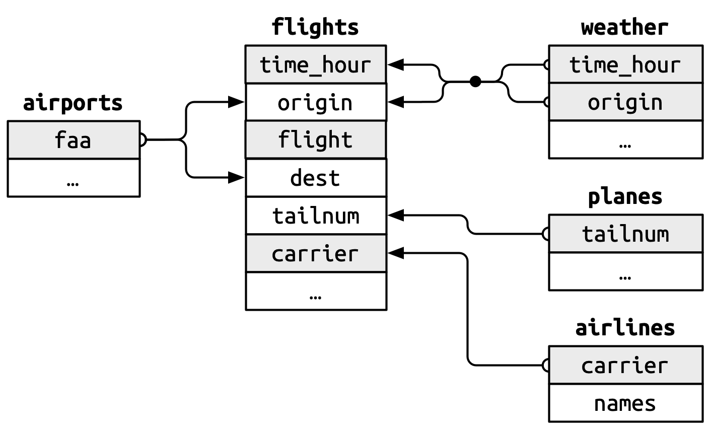
Note: grey shading indicates the primary key for that particular dataset.

• flights$origin –> airports$faa
• flights$dest –> airports$faa
• flights$origin-flights$time_hour –> weather$origin-weather$time_hour.
• flights$tailnum –> planes$tailnum
• flights$carrier –> airlines$carrier

Checking Keys

A nice feature of these data are that the primary and foreign keys have the same name and almost every variable name used across multiple tables has the same meaning.¹ This isn’t always the case!²

It is good practice to make sure your primary keys actually uniquely identify an observation and that they don’t have any missing values.

planes |> 
  count(tailnum) |>
  filter(n > 1)

1

If your primary keys uniquely identify each observation you’ll get an empty tibble in return.

# A tibble: 0 × 2
# ℹ 2 variables: tailnum <chr>, n <int>

planes |> 
  filter(is.na(tailnum))

2

If none of your primary keys are missing you’ll get an empty tibble in return here too.

# A tibble: 0 × 9
# ℹ 9 variables: tailnum <chr>, year <int>, type <chr>, manufacturer <chr>,
#   model <chr>, engines <int>, seats <int>, speed <int>, engine <chr>

1. With the exception of year: it means year of departure in flights and year of manufacture in planes.

2. We’ll cover how to handle this shortly.

Surrogate Keys

Sometimes you’ll want to create an index of your observations to serve as a surrogate key because the compound primary key is not particlarly easy to reference.

For example, our flights dataset has three variables that uniquely identify each observation: time_hour, carrier, flight.

flights2 <- flights |> 
  mutate(id = row_number(), .before = 1)
flights2

3

row_number() simply specifies the row number of the dataframe.

# A tibble: 336,776 × 20
      id  year month   day dep_time sched_dep_time dep_delay arr_time
   <int> <int> <int> <int>    <int>          <int>     <dbl>    <int>
 1     1  2013     1     1      517            515         2      830
 2     2  2013     1     1      533            529         4      850
 3     3  2013     1     1      542            540         2      923
 4     4  2013     1     1      544            545        -1     1004
 5     5  2013     1     1      554            600        -6      812
 6     6  2013     1     1      554            558        -4      740
 7     7  2013     1     1      555            600        -5      913
 8     8  2013     1     1      557            600        -3      709
 9     9  2013     1     1      557            600        -3      838
10    10  2013     1     1      558            600        -2      753
# ℹ 336,766 more rows
# ℹ 12 more variables: sched_arr_time <int>, arr_delay <dbl>, carrier <chr>,
#   flight <int>, tailnum <chr>, origin <chr>, dest <chr>, air_time <dbl>,
#   distance <dbl>, hour <dbl>, minute <dbl>, time_hour <dttm>

Basic (Equi-) Joins

All join functions have the same basic interface: they take a pair of data frames and return one data frame.

The order of the rows and columns is primarily going to be determined by the first data frame.

dplyr has two types of joins: mutating and filtering.

Mutating Joins

Add new variables to one data frame from matching observations from another data frame.

• left_join()
• right_join()
• inner_join()
• full_join()

Filtering Joins

Filter observations from one data frame based on whether or not they match an observation in another data frame.

• semi_join()
• anti-join()

Mutating Joins

left_join()

• The most common type of join
• Appends columns from y to x by the rows in x
  • NA added if there is nothing from y
• Natural join: when all variables that appear in both datasets are used as the join key
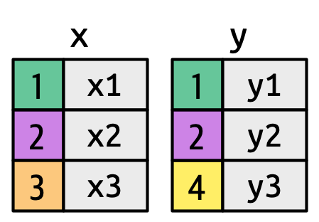
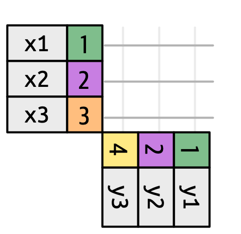
  • If the join_by() argument is not specified, left_join() will automatically join by all columns that have names and values in common.

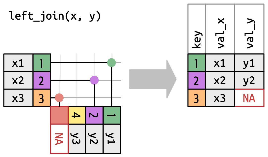
left_join in nycflights13

flights2 <- flights |> 
  select(year, time_hour, origin, dest, tailnum, carrier)

With only the pertinent variables from the flights dataset, we can see how a left_join works with the airlines dataset.

flights2 |>
  left_join(airlines)

Joining with `by = join_by(carrier)`

# A tibble: 336,776 × 7
    year time_hour           origin dest  tailnum carrier name                  
   <int> <dttm>              <chr>  <chr> <chr>   <chr>   <chr>                 
 1  2013 2013-01-01 05:00:00 EWR    IAH   N14228  UA      United Air Lines Inc. 
 2  2013 2013-01-01 05:00:00 LGA    IAH   N24211  UA      United Air Lines Inc. 
 3  2013 2013-01-01 05:00:00 JFK    MIA   N619AA  AA      American Airlines Inc.
 4  2013 2013-01-01 05:00:00 JFK    BQN   N804JB  B6      JetBlue Airways       
 5  2013 2013-01-01 06:00:00 LGA    ATL   N668DN  DL      Delta Air Lines Inc.  
 6  2013 2013-01-01 05:00:00 EWR    ORD   N39463  UA      United Air Lines Inc. 
 7  2013 2013-01-01 06:00:00 EWR    FLL   N516JB  B6      JetBlue Airways       
 8  2013 2013-01-01 06:00:00 LGA    IAD   N829AS  EV      ExpressJet Airlines I…
 9  2013 2013-01-01 06:00:00 JFK    MCO   N593JB  B6      JetBlue Airways       
10  2013 2013-01-01 06:00:00 LGA    ORD   N3ALAA  AA      American Airlines Inc.
# ℹ 336,766 more rows

Different variable meanings

flights2 |> 
  left_join(planes)

Joining with `by = join_by(year, tailnum)`

# A tibble: 336,776 × 13
    year time_hour           origin dest  tailnum carrier type  manufacturer
   <int> <dttm>              <chr>  <chr> <chr>   <chr>   <chr> <chr>       
 1  2013 2013-01-01 05:00:00 EWR    IAH   N14228  UA      <NA>  <NA>        
 2  2013 2013-01-01 05:00:00 LGA    IAH   N24211  UA      <NA>  <NA>        
 3  2013 2013-01-01 05:00:00 JFK    MIA   N619AA  AA      <NA>  <NA>        
 4  2013 2013-01-01 05:00:00 JFK    BQN   N804JB  B6      <NA>  <NA>        
 5  2013 2013-01-01 06:00:00 LGA    ATL   N668DN  DL      <NA>  <NA>        
 6  2013 2013-01-01 05:00:00 EWR    ORD   N39463  UA      <NA>  <NA>        
 7  2013 2013-01-01 06:00:00 EWR    FLL   N516JB  B6      <NA>  <NA>        
 8  2013 2013-01-01 06:00:00 LGA    IAD   N829AS  EV      <NA>  <NA>        
 9  2013 2013-01-01 06:00:00 JFK    MCO   N593JB  B6      <NA>  <NA>        
10  2013 2013-01-01 06:00:00 LGA    ORD   N3ALAA  AA      <NA>  <NA>        
# ℹ 336,766 more rows
# ℹ 5 more variables: model <chr>, engines <int>, seats <int>, speed <int>,
#   engine <chr>

When we try to do this, however, we get a bunch of NAs. Why?

Different variable meanings

flights2 |> 
  left_join(planes)

Joining with `by = join_by(year, tailnum)`

# A tibble: 336,776 × 13
    year time_hour           origin dest  tailnum carrier type  manufacturer
   <int> <dttm>              <chr>  <chr> <chr>   <chr>   <chr> <chr>       
 1  2013 2013-01-01 05:00:00 EWR    IAH   N14228  UA      <NA>  <NA>        
 2  2013 2013-01-01 05:00:00 LGA    IAH   N24211  UA      <NA>  <NA>        
 3  2013 2013-01-01 05:00:00 JFK    MIA   N619AA  AA      <NA>  <NA>        
 4  2013 2013-01-01 05:00:00 JFK    BQN   N804JB  B6      <NA>  <NA>        
 5  2013 2013-01-01 06:00:00 LGA    ATL   N668DN  DL      <NA>  <NA>        
 6  2013 2013-01-01 05:00:00 EWR    ORD   N39463  UA      <NA>  <NA>        
 7  2013 2013-01-01 06:00:00 EWR    FLL   N516JB  B6      <NA>  <NA>        
 8  2013 2013-01-01 06:00:00 LGA    IAD   N829AS  EV      <NA>  <NA>        
 9  2013 2013-01-01 06:00:00 JFK    MCO   N593JB  B6      <NA>  <NA>        
10  2013 2013-01-01 06:00:00 LGA    ORD   N3ALAA  AA      <NA>  <NA>        
# ℹ 336,766 more rows
# ℹ 5 more variables: model <chr>, engines <int>, seats <int>, speed <int>,
#   engine <chr>

Join is trying to use tailnum and year as a compound key. While both datasets have year as a variable, they mean different things. Therefore, we need to be explicit here about what to join by.

Different variable meanings

flights2 |> 
  left_join(planes, join_by(tailnum))

4

join_by(tailnum) is short for join_by(tailnum == tailnum) making these types of basic joins equi joins.

# A tibble: 336,776 × 14
   year.x time_hour           origin dest  tailnum carrier year.y type          
    <int> <dttm>              <chr>  <chr> <chr>   <chr>    <int> <chr>         
 1   2013 2013-01-01 05:00:00 EWR    IAH   N14228  UA        1999 Fixed wing mu…
 2   2013 2013-01-01 05:00:00 LGA    IAH   N24211  UA        1998 Fixed wing mu…
 3   2013 2013-01-01 05:00:00 JFK    MIA   N619AA  AA        1990 Fixed wing mu…
 4   2013 2013-01-01 05:00:00 JFK    BQN   N804JB  B6        2012 Fixed wing mu…
 5   2013 2013-01-01 06:00:00 LGA    ATL   N668DN  DL        1991 Fixed wing mu…
 6   2013 2013-01-01 05:00:00 EWR    ORD   N39463  UA        2012 Fixed wing mu…
 7   2013 2013-01-01 06:00:00 EWR    FLL   N516JB  B6        2000 Fixed wing mu…
 8   2013 2013-01-01 06:00:00 LGA    IAD   N829AS  EV        1998 Fixed wing mu…
 9   2013 2013-01-01 06:00:00 JFK    MCO   N593JB  B6        2004 Fixed wing mu…
10   2013 2013-01-01 06:00:00 LGA    ORD   N3ALAA  AA          NA <NA>          
# ℹ 336,766 more rows
# ℹ 6 more variables: manufacturer <chr>, model <chr>, engines <int>,
#   seats <int>, speed <int>, engine <chr>

When you have the same variable name but they mean different things you can specify a particular suffix with the suffix argument.

Different variable names

If you have keys that have the same meaning (values) but are named different things in their respective datasets you’d also specify that with join_by()

flights2 |> 
  left_join(airports, join_by(dest == faa))

5

by = c("dest" = "faa") was the former syntax for this and you still might see that in older code.

# A tibble: 336,776 × 13
    year time_hour           origin dest  tailnum carrier name         lat   lon
   <int> <dttm>              <chr>  <chr> <chr>   <chr>   <chr>      <dbl> <dbl>
 1  2013 2013-01-01 05:00:00 EWR    IAH   N14228  UA      George Bu…  30.0 -95.3
 2  2013 2013-01-01 05:00:00 LGA    IAH   N24211  UA      George Bu…  30.0 -95.3
 3  2013 2013-01-01 05:00:00 JFK    MIA   N619AA  AA      Miami Intl  25.8 -80.3
 4  2013 2013-01-01 05:00:00 JFK    BQN   N804JB  B6      <NA>        NA    NA  
 5  2013 2013-01-01 06:00:00 LGA    ATL   N668DN  DL      Hartsfiel…  33.6 -84.4
 6  2013 2013-01-01 05:00:00 EWR    ORD   N39463  UA      Chicago O…  42.0 -87.9
 7  2013 2013-01-01 06:00:00 EWR    FLL   N516JB  B6      Fort Laud…  26.1 -80.2
 8  2013 2013-01-01 06:00:00 LGA    IAD   N829AS  EV      Washingto…  38.9 -77.5
 9  2013 2013-01-01 06:00:00 JFK    MCO   N593JB  B6      Orlando I…  28.4 -81.3
10  2013 2013-01-01 06:00:00 LGA    ORD   N3ALAA  AA      Chicago O…  42.0 -87.9
# ℹ 336,766 more rows
# ℹ 4 more variables: alt <dbl>, tz <dbl>, dst <chr>, tzone <chr>

This will match dest to faa for the join and then drop faa.

Different variable names

You can request dplyr to keep both keys with keep = TRUE argument.

flights2 |> 
  left_join(airports, join_by(dest == faa), keep = TRUE) 

# A tibble: 336,776 × 14
    year time_hour           origin dest  tailnum carrier faa   name         lat
   <int> <dttm>              <chr>  <chr> <chr>   <chr>   <chr> <chr>      <dbl>
 1  2013 2013-01-01 05:00:00 EWR    IAH   N14228  UA      IAH   George Bu…  30.0
 2  2013 2013-01-01 05:00:00 LGA    IAH   N24211  UA      IAH   George Bu…  30.0
 3  2013 2013-01-01 05:00:00 JFK    MIA   N619AA  AA      MIA   Miami Intl  25.8
 4  2013 2013-01-01 05:00:00 JFK    BQN   N804JB  B6      <NA>  <NA>        NA  
 5  2013 2013-01-01 06:00:00 LGA    ATL   N668DN  DL      ATL   Hartsfiel…  33.6
 6  2013 2013-01-01 05:00:00 EWR    ORD   N39463  UA      ORD   Chicago O…  42.0
 7  2013 2013-01-01 06:00:00 EWR    FLL   N516JB  B6      FLL   Fort Laud…  26.1
 8  2013 2013-01-01 06:00:00 LGA    IAD   N829AS  EV      IAD   Washingto…  38.9
 9  2013 2013-01-01 06:00:00 JFK    MCO   N593JB  B6      MCO   Orlando I…  28.4
10  2013 2013-01-01 06:00:00 LGA    ORD   N3ALAA  AA      ORD   Chicago O…  42.0
# ℹ 336,766 more rows
# ℹ 5 more variables: lon <dbl>, alt <dbl>, tz <dbl>, dst <chr>, tzone <chr>

right_join()

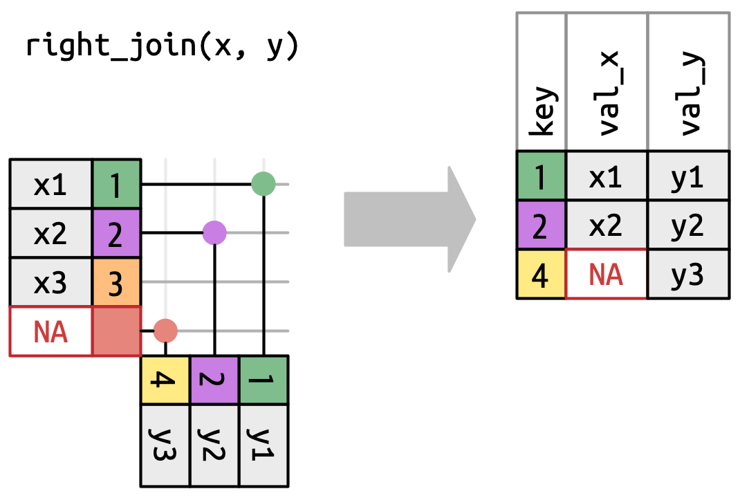
Has the same interface as a left_join but keeps all rows in y instead of x

inner_join()

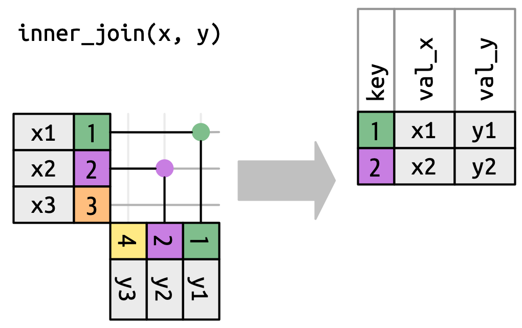
Has the same interface as a left_join but only keeps rows that occur in both x and y

full_join()

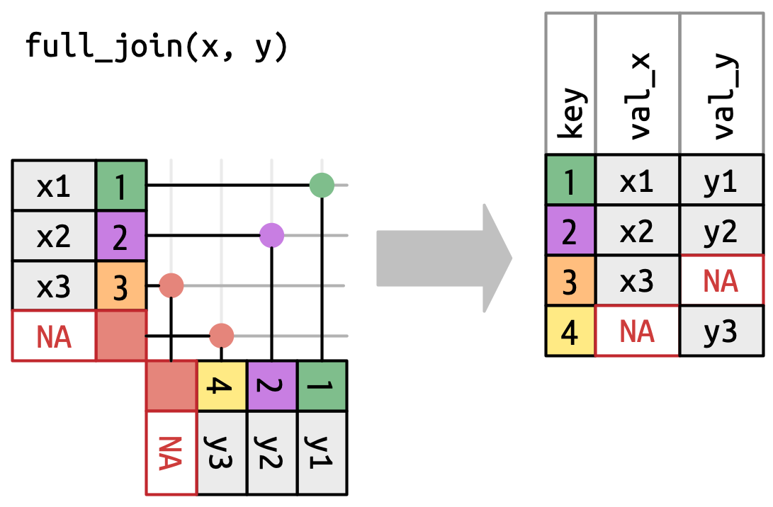
Has the same interface as a left_join but keeps all rows in either x or y

Filtering Joins

semi_join()

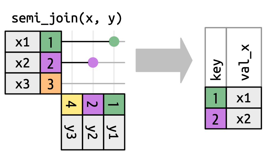
Keeps all rows in x that have a match in y

semi_join() in nycflights13

We could use a semi-join to filter the airports dataset to show just the origin airports.

airports |> 
  semi_join(flights2, join_by(faa == origin))

# A tibble: 3 × 8
  faa   name                  lat   lon   alt    tz dst   tzone           
  <chr> <chr>               <dbl> <dbl> <dbl> <dbl> <chr> <chr>           
1 EWR   Newark Liberty Intl  40.7 -74.2    18    -5 A     America/New_York
2 JFK   John F Kennedy Intl  40.6 -73.8    13    -5 A     America/New_York
3 LGA   La Guardia           40.8 -73.9    22    -5 A     America/New_York

anti_join()

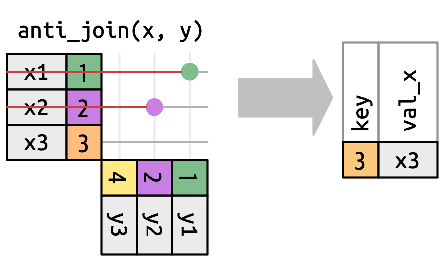
Returns all rows in x that don’t have a match in y

anti_join() in nycflights13

We can find rows that are missing from airports by looking for flights that don’t have a matching destination airport.

airports |> 
  anti_join(flights2, join_by(faa == origin))

# A tibble: 1,455 × 8
   faa   name                             lat    lon   alt    tz dst   tzone    
   <chr> <chr>                          <dbl>  <dbl> <dbl> <dbl> <chr> <chr>    
 1 04G   Lansdowne Airport               41.1  -80.6  1044    -5 A     America/…
 2 06A   Moton Field Municipal Airport   32.5  -85.7   264    -6 A     America/…
 3 06C   Schaumburg Regional             42.0  -88.1   801    -6 A     America/…
 4 06N   Randall Airport                 41.4  -74.4   523    -5 A     America/…
 5 09J   Jekyll Island Airport           31.1  -81.4    11    -5 A     America/…
 6 0A9   Elizabethton Municipal Airport  36.4  -82.2  1593    -5 A     America/…
 7 0G6   Williams County Airport         41.5  -84.5   730    -5 A     America/…
 8 0G7   Finger Lakes Regional Airport   42.9  -76.8   492    -5 A     America/…
 9 0P2   Shoestring Aviation Airfield    39.8  -76.6  1000    -5 U     America/…
10 0S9   Jefferson County Intl           48.1 -123.    108    -8 A     America/…
# ℹ 1,445 more rows

This type of join is useful for finding missing values that are implicit in the data (i.e. NAs that don’t show up in the data but only exist as an absence.)

More Than One Match

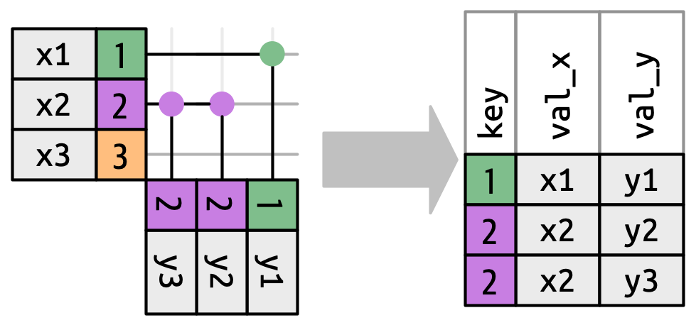
There are three possible outcomes for a row in x:

• If it doesn’t match anything, it’s dropped.
• If it matches 1 row in y, it’s preserved.
• If it matches more than 1 row in y, it’s duplicated once for each match.

What happens if we match on more than one row?

More Than One Match

df1 <- tibble(key = c(1, 2, 2), val_x = c("x1", "x2", "x3"))
df2 <- tibble(key = c(1, 2, 2), val_y = c("y1", "y2", "y3"))

df1 |> 
  inner_join(df2, join_by(key))

Warning in inner_join(df1, df2, join_by(key)): Detected an unexpected many-to-many relationship between `x` and `y`.
ℹ Row 2 of `x` matches multiple rows in `y`.
ℹ Row 2 of `y` matches multiple rows in `x`.
ℹ If a many-to-many relationship is expected, set `relationship =
  "many-to-many"` to silence this warning.

# A tibble: 5 × 3
    key val_x val_y
  <dbl> <chr> <chr>
1     1 x1    y1   
2     2 x2    y2   
3     2 x2    y3   
4     2 x3    y2   
5     2 x3    y3   

If you’re doing this deliberately, set relationship = “many-to-many”, as the warning suggests.

Given their nature, filtering joins never duplicate rows like mutating joins do. They will only ever return a subset of the datasets.

Non-Equi Joins

The joins we’ve discussed thus far have all been equi-joins, where the rows match if the x key equals the y key. But you can also specify other types of relationships.

dplyr has four different types of non-equi joins:

• Cross joins match every pair of rows.

Cross joins, aka self-joins, are useful when generating permutations (e.g. creating every possible combination of values). This comes in handy when creating datasets of predicted probabilities for plotting in ggplot.

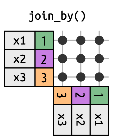
Non-Equi Joins

The joins we’ve discussed thus far have all been equi-joins, where the rows match if the x key equals the y key. But you can also specify other types of relationships.

dplyr has four different types of non-equi joins:

• Cross joins match every pair of rows.
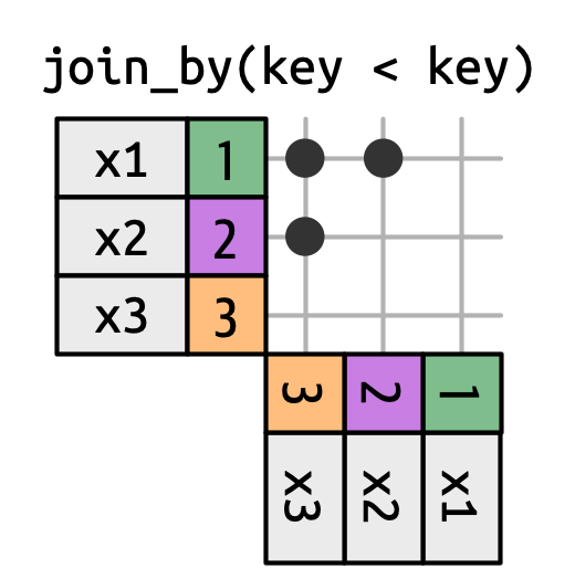
• Inequality joins use <, <=, >, and >= instead of ==.
  • Overlap joins are a special type of inequality join designed to work with ranges¹.

Inequality joins can be used to restrict the cross join so that instead of generating all permutations, we generate all combinations.

1. Overlap joins provide three helpers that use inequality joins to make it easier to work with intervals: between(), within(), overlaps(). Read more about their functionality and specifications here.

Non-Equi Joins

The joins we’ve discussed thus far have all been equi-joins, where the rows match if the x key equals the y key. But you can also specify other types of relationships.

dplyr has four different types of non-equi joins:

• Cross joins match every pair of rows.
• Inequality joins use <, <=, >, and >= instead of ==.
  • Overlap joins are a special type of inequality join designed to work with ranges.
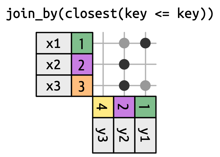
• Rolling joins are similar to inequality joins but only find the closest match.

Rolling joins are a special type of inequality join where instead of getting every row that satisfies the inequality, you get just the closest row. You can turn any inequality join into a rolling join by adding closest().

Tidying and Reshaping Data

What is Tidy Data

Tidy data¹ (aka “long data”) are such that:

1. The values for a single variable are in their own column.
2. The values for a single observation are in their own row.
3. There is only one value per cell.

1. Read the original article here.

Why do we Want Tidy Data?

• Easier to understand many rows than many columns¹
• Required for plotting in ggplot2²
• Required for many types of statistical procedures (e.g. hierarchical or mixed effects models)
• Fewer issues with missing values and “imbalanced” repeated measures data
• Having a consistent method for storing data means it’s easier to learn the tools to work with it since there’s an underlying uniformity.

Most real-world data is not tidy because data are often organized for goals other than analysis (i.e. data entry) and most people aren’t familiar with the principles of tidy data.

1. Placing variables in columns also leverages R’s vectorized nature, i.e. most built-in R functions work with values of vectors.

2. In fact, all tidyverse functions are designed to work with tidy data.

Slightly “Messy” Data

Program	First Year	Second Year
Evans School	10	6
Arts & Sciences	5	6
Public Health	2	3
Other	5	1

• What is an observation?
  • A group of students from a program of a given year
• What are the variables?
  • Program, Year
• What are the values?
  • Program: Evans School, Arts & Sciences, Public Health, Other
  • Year: First, Second – in column headings. Bad!
  • Count: spread over two columns!

Tidy Version

Program	Year	Count
Evans School	First	10
Evans School	Second	6
Arts & Sciences	First	5
Arts & Sciences	Second	6
Public Health	First	2
Public Health	Second	3
Other	First	5
Other	Second	1

• Each variable is a column.

• Each observation is a row.

• Each cell has a single value.

Billboard Data

Rows: 317
Columns: 81
$ year         <int> 2000, 2000, 2000, 2000, 2000, 2000, 2000, 2000, 2000, 200…
$ artist       <chr> "2 Pac", "2Ge+her", "3 Doors Down", "3 Doors Down", "504 …
$ track        <chr> "Baby Don't Cry (Keep...", "The Hardest Part Of ...", "Kr…
$ time         <time> 04:22:00, 03:15:00, 03:53:00, 04:24:00, 03:35:00, 03:24:…
$ date.entered <date> 2000-02-26, 2000-09-02, 2000-04-08, 2000-10-21, 2000-04-…
$ wk1          <int> 87, 91, 81, 76, 57, 51, 97, 84, 59, 76, 84, 57, 50, 71, 7…
$ wk2          <int> 82, 87, 70, 76, 34, 39, 97, 62, 53, 76, 84, 47, 39, 51, 6…
$ wk3          <int> 72, 92, 68, 72, 25, 34, 96, 51, 38, 74, 75, 45, 30, 28, 5…
$ wk4          <int> 77, NA, 67, 69, 17, 26, 95, 41, 28, 69, 73, 29, 28, 18, 4…
$ wk5          <int> 87, NA, 66, 67, 17, 26, 100, 38, 21, 68, 73, 23, 21, 13, …
$ wk6          <int> 94, NA, 57, 65, 31, 19, NA, 35, 18, 67, 69, 18, 19, 13, 3…
$ wk7          <int> 99, NA, 54, 55, 36, 2, NA, 35, 16, 61, 68, 11, 20, 11, 34…
$ wk8          <int> NA, NA, 53, 59, 49, 2, NA, 38, 14, 58, 65, 9, 17, 1, 29, …
$ wk9          <int> NA, NA, 51, 62, 53, 3, NA, 38, 12, 57, 73, 9, 17, 1, 27, …
$ wk10         <int> NA, NA, 51, 61, 57, 6, NA, 36, 10, 59, 83, 11, 17, 2, 30,…
$ wk11         <int> NA, NA, 51, 61, 64, 7, NA, 37, 9, 66, 92, 1, 17, 2, 36, N…
$ wk12         <int> NA, NA, 51, 59, 70, 22, NA, 37, 8, 68, NA, 1, 3, 3, 37, N…
$ wk13         <int> NA, NA, 47, 61, 75, 29, NA, 38, 6, 61, NA, 1, 3, 3, 39, N…
$ wk14         <int> NA, NA, 44, 66, 76, 36, NA, 49, 1, 67, NA, 1, 7, 4, 49, N…
$ wk15         <int> NA, NA, 38, 72, 78, 47, NA, 61, 2, 59, NA, 4, 10, 12, 57,…
$ wk16         <int> NA, NA, 28, 76, 85, 67, NA, 63, 2, 63, NA, 8, 17, 11, 63,…
$ wk17         <int> NA, NA, 22, 75, 92, 66, NA, 62, 2, 67, NA, 12, 25, 13, 65…
$ wk18         <int> NA, NA, 18, 67, 96, 84, NA, 67, 2, 71, NA, 22, 29, 15, 68…
$ wk19         <int> NA, NA, 18, 73, NA, 93, NA, 83, 3, 79, NA, 23, 29, 18, 79…
$ wk20         <int> NA, NA, 14, 70, NA, 94, NA, 86, 4, 89, NA, 43, 40, 20, 86…
$ wk21         <int> NA, NA, 12, NA, NA, NA, NA, NA, 5, NA, NA, 44, 43, 30, NA…
$ wk22         <int> NA, NA, 7, NA, NA, NA, NA, NA, 5, NA, NA, NA, 50, 40, NA,…
$ wk23         <int> NA, NA, 6, NA, NA, NA, NA, NA, 6, NA, NA, NA, NA, 39, NA,…
$ wk24         <int> NA, NA, 6, NA, NA, NA, NA, NA, 9, NA, NA, NA, NA, 44, NA,…
$ wk25         <int> NA, NA, 6, NA, NA, NA, NA, NA, 13, NA, NA, NA, NA, NA, NA…
$ wk26         <int> NA, NA, 5, NA, NA, NA, NA, NA, 14, NA, NA, NA, NA, NA, NA…
$ wk27         <int> NA, NA, 5, NA, NA, NA, NA, NA, 16, NA, NA, NA, NA, NA, NA…
$ wk28         <int> NA, NA, 4, NA, NA, NA, NA, NA, 23, NA, NA, NA, NA, NA, NA…
$ wk29         <int> NA, NA, 4, NA, NA, NA, NA, NA, 22, NA, NA, NA, NA, NA, NA…
$ wk30         <int> NA, NA, 4, NA, NA, NA, NA, NA, 33, NA, NA, NA, NA, NA, NA…
$ wk31         <int> NA, NA, 4, NA, NA, NA, NA, NA, 36, NA, NA, NA, NA, NA, NA…
$ wk32         <int> NA, NA, 3, NA, NA, NA, NA, NA, 43, NA, NA, NA, NA, NA, NA…
$ wk33         <int> NA, NA, 3, NA, NA, NA, NA, NA, NA, NA, NA, NA, NA, NA, NA…
$ wk34         <int> NA, NA, 3, NA, NA, NA, NA, NA, NA, NA, NA, NA, NA, NA, NA…
$ wk35         <int> NA, NA, 4, NA, NA, NA, NA, NA, NA, NA, NA, NA, NA, NA, NA…
$ wk36         <int> NA, NA, 5, NA, NA, NA, NA, NA, NA, NA, NA, NA, NA, NA, NA…
$ wk37         <int> NA, NA, 5, NA, NA, NA, NA, NA, NA, NA, NA, NA, NA, NA, NA…
$ wk38         <int> NA, NA, 9, NA, NA, NA, NA, NA, NA, NA, NA, NA, NA, NA, NA…
$ wk39         <int> NA, NA, 9, NA, NA, NA, NA, NA, NA, NA, NA, NA, NA, NA, NA…
$ wk40         <int> NA, NA, 15, NA, NA, NA, NA, NA, NA, NA, NA, NA, NA, NA, N…
$ wk41         <int> NA, NA, 14, NA, NA, NA, NA, NA, NA, NA, NA, NA, NA, NA, N…
$ wk42         <int> NA, NA, 13, NA, NA, NA, NA, NA, NA, NA, NA, NA, NA, NA, N…
$ wk43         <int> NA, NA, 14, NA, NA, NA, NA, NA, NA, NA, NA, NA, NA, NA, N…
$ wk44         <int> NA, NA, 16, NA, NA, NA, NA, NA, NA, NA, NA, NA, NA, NA, N…
$ wk45         <int> NA, NA, 17, NA, NA, NA, NA, NA, NA, NA, NA, NA, NA, NA, N…
$ wk46         <int> NA, NA, 21, NA, NA, NA, NA, NA, NA, NA, NA, NA, NA, NA, N…
$ wk47         <int> NA, NA, 22, NA, NA, NA, NA, NA, NA, NA, NA, NA, NA, NA, N…
$ wk48         <int> NA, NA, 24, NA, NA, NA, NA, NA, NA, NA, NA, NA, NA, NA, N…
$ wk49         <int> NA, NA, 28, NA, NA, NA, NA, NA, NA, NA, NA, NA, NA, NA, N…
$ wk50         <int> NA, NA, 33, NA, NA, NA, NA, NA, NA, NA, NA, NA, NA, NA, N…
$ wk51         <int> NA, NA, 42, NA, NA, NA, NA, NA, NA, NA, NA, NA, NA, NA, N…
$ wk52         <int> NA, NA, 42, NA, NA, NA, NA, NA, NA, NA, NA, NA, NA, NA, N…
$ wk53         <int> NA, NA, 49, NA, NA, NA, NA, NA, NA, NA, NA, NA, NA, NA, N…
$ wk54         <int> NA, NA, NA, NA, NA, NA, NA, NA, NA, NA, NA, NA, NA, NA, N…
$ wk55         <int> NA, NA, NA, NA, NA, NA, NA, NA, NA, NA, NA, NA, NA, NA, N…
$ wk56         <int> NA, NA, NA, NA, NA, NA, NA, NA, NA, NA, NA, NA, NA, NA, N…
$ wk57         <int> NA, NA, NA, NA, NA, NA, NA, NA, NA, NA, NA, NA, NA, NA, N…
$ wk58         <int> NA, NA, NA, NA, NA, NA, NA, NA, NA, NA, NA, NA, NA, NA, N…
$ wk59         <int> NA, NA, NA, NA, NA, NA, NA, NA, NA, NA, NA, NA, NA, NA, N…
$ wk60         <int> NA, NA, NA, NA, NA, NA, NA, NA, NA, NA, NA, NA, NA, NA, N…
$ wk61         <int> NA, NA, NA, NA, NA, NA, NA, NA, NA, NA, NA, NA, NA, NA, N…
$ wk62         <int> NA, NA, NA, NA, NA, NA, NA, NA, NA, NA, NA, NA, NA, NA, N…
$ wk63         <int> NA, NA, NA, NA, NA, NA, NA, NA, NA, NA, NA, NA, NA, NA, N…
$ wk64         <int> NA, NA, NA, NA, NA, NA, NA, NA, NA, NA, NA, NA, NA, NA, N…
$ wk65         <int> NA, NA, NA, NA, NA, NA, NA, NA, NA, NA, NA, NA, NA, NA, N…
$ wk66         <int> NA, NA, NA, NA, NA, NA, NA, NA, NA, NA, NA, NA, NA, NA, N…
$ wk67         <int> NA, NA, NA, NA, NA, NA, NA, NA, NA, NA, NA, NA, NA, NA, N…
$ wk68         <int> NA, NA, NA, NA, NA, NA, NA, NA, NA, NA, NA, NA, NA, NA, N…
$ wk69         <int> NA, NA, NA, NA, NA, NA, NA, NA, NA, NA, NA, NA, NA, NA, N…
$ wk70         <int> NA, NA, NA, NA, NA, NA, NA, NA, NA, NA, NA, NA, NA, NA, N…
$ wk71         <int> NA, NA, NA, NA, NA, NA, NA, NA, NA, NA, NA, NA, NA, NA, N…
$ wk72         <int> NA, NA, NA, NA, NA, NA, NA, NA, NA, NA, NA, NA, NA, NA, N…
$ wk73         <int> NA, NA, NA, NA, NA, NA, NA, NA, NA, NA, NA, NA, NA, NA, N…
$ wk74         <int> NA, NA, NA, NA, NA, NA, NA, NA, NA, NA, NA, NA, NA, NA, N…
$ wk75         <int> NA, NA, NA, NA, NA, NA, NA, NA, NA, NA, NA, NA, NA, NA, N…
$ wk76         <int> NA, NA, NA, NA, NA, NA, NA, NA, NA, NA, NA, NA, NA, NA, N…

This data is just ugly-messy!

Week columns continue up to wk76!

How is Billboard currently organized?

• What are the observations in the data?
  • Song on the Billboard chart each week
• What are the variables in the data?
  • Year, artist, track, song length, date entered Hot 100, week since first entered Hot 100 (spread over many columns), rank during week (spread over many columns)
• What are the values in the data?
  • e.g. 2000; 3 Doors Down; Kryptonite; 3 minutes 53 seconds; April 8, 2000; Week 3 (stuck in column headings); rank 68 (spread over many columns)

tidyr

The tidyr package provides functions to tidy up data.

Key functions:

• pivot_longer(): takes a set of columns and pivots them down (“longer”) to make two new columns (which you can name yourself):
  • A name column that stores the original column names
  • A value with the values in those original columns

• pivot_wider(): inverts pivot_longer() by taking two columns and pivoting them up and across (“wider”) into multiple columns

pivot_longer()

This function usually takes three arguments:

1. cols: The columns that need to be pivoted (are not variables)
2. names_to: Names the new variable that is stored in multiple columns
3. values_to: Names the variable stored in the cell values

pivot_longer()

This function usually takes three arguments:

1. cols: The columns that need to be pivoted (are not variables)
2. names_to: Names the new variable that is stored in multiple columns
3. values_to: Names the variable stored in the cell values

pivot_longer()

This function usually takes three arguments:

1. cols: The columns that need to be pivoted (are not variables)
2. names_to: Names the new variable that is stored in multiple columns
3. values_to: Names the variable stored in the cell values

pivot_longer()

This function usually takes three arguments:

1. cols: The columns that need to be pivoted (are not variables)
2. names_to: Names the new variable that is stored in multiple columns
3. values_to: Names the variable stored in the cell values

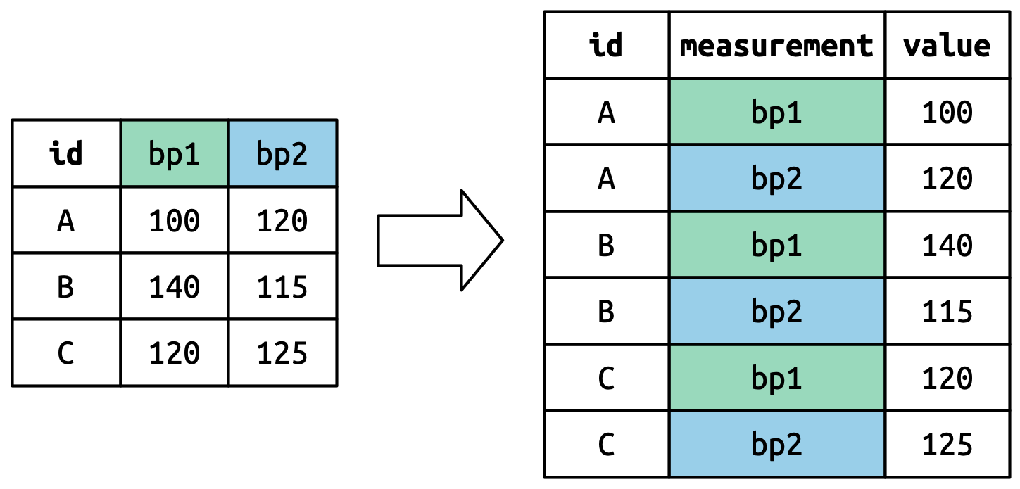
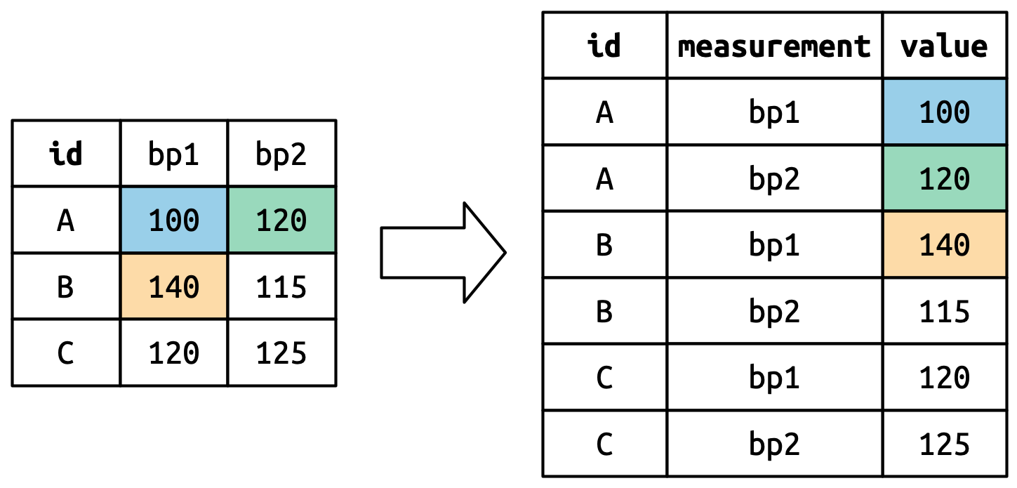
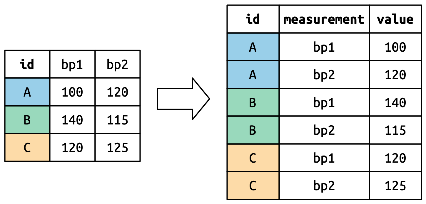
pivot_longer() Example

billboard_2000 <- billboard_2000_raw |> 
  pivot_longer(cols = starts_with("wk"),
               names_to ="week",
               values_to = "rank")

billboard_2000 |> head(10)

1

starts_with() is one of the helper functions from tidyselect that helps select certain common patterns. We could have also used cols = wk1:wk76.

# A tibble: 10 × 7
    year artist track                   time   date.entered week   rank
   <int> <chr>  <chr>                   <time> <date>       <chr> <int>
 1  2000 2 Pac  Baby Don't Cry (Keep... 04:22  2000-02-26   wk1      87
 2  2000 2 Pac  Baby Don't Cry (Keep... 04:22  2000-02-26   wk2      82
 3  2000 2 Pac  Baby Don't Cry (Keep... 04:22  2000-02-26   wk3      72
 4  2000 2 Pac  Baby Don't Cry (Keep... 04:22  2000-02-26   wk4      77
 5  2000 2 Pac  Baby Don't Cry (Keep... 04:22  2000-02-26   wk5      87
 6  2000 2 Pac  Baby Don't Cry (Keep... 04:22  2000-02-26   wk6      94
 7  2000 2 Pac  Baby Don't Cry (Keep... 04:22  2000-02-26   wk7      99
 8  2000 2 Pac  Baby Don't Cry (Keep... 04:22  2000-02-26   wk8      NA
 9  2000 2 Pac  Baby Don't Cry (Keep... 04:22  2000-02-26   wk9      NA
10  2000 2 Pac  Baby Don't Cry (Keep... 04:22  2000-02-26   wk10     NA

Now we have a single week column!

Lots of Missing Values?!

glimpse(billboard_2000)

Rows: 24,092
Columns: 7
$ year         <int> 2000, 2000, 2000, 2000, 2000, 2000, 2000, 2000, 2000, 200…
$ artist       <chr> "2 Pac", "2 Pac", "2 Pac", "2 Pac", "2 Pac", "2 Pac", "2 …
$ track        <chr> "Baby Don't Cry (Keep...", "Baby Don't Cry (Keep...", "Ba…
$ time         <time> 04:22:00, 04:22:00, 04:22:00, 04:22:00, 04:22:00, 04:22:…
$ date.entered <date> 2000-02-26, 2000-02-26, 2000-02-26, 2000-02-26, 2000-02-…
$ week         <chr> "wk1", "wk2", "wk3", "wk4", "wk5", "wk6", "wk7", "wk8", "…
$ rank         <int> 87, 82, 72, 77, 87, 94, 99, NA, NA, NA, NA, NA, NA, NA, N…

It looks like 2 Pac’s song “Baby Don’t Cry” was only on the Billboard Hot 100 for 7 weeks and then dropped off the charts.

summary(billboard_2000$rank)

   Min. 1st Qu.  Median    Mean 3rd Qu.    Max.    NA's 
   1.00   26.00   51.00   51.05   76.00  100.00   18785 

We don’t want to keep the 18785 rows with missing ranks.

Pivoting Better: values_drop_na

Adding the argument values_drop_na = TRUE to pivot_longer() will remove rows with missing ranks. Since these NAs don’t really represent unknown observations (i.e. they were forced to exist by the structure of the dataset) this is an appropriate approach here.

billboard_2000 <- billboard_2000_raw %>%
  pivot_longer(cols = wk1:wk76, 
               names_to = "week", 
               values_to = "rank", 
               values_drop_na = TRUE)
summary(billboard_2000$rank)

   Min. 1st Qu.  Median    Mean 3rd Qu.    Max. 
   1.00   26.00   51.00   51.05   76.00  100.00 

No more NA values!

dim(billboard_2000)

[1] 5307    7

And way fewer rows!

parse_number()

The week column is of the type character, but it should be numeric.

head(billboard_2000$week)

[1] "wk1" "wk2" "wk3" "wk4" "wk5" "wk6"

parse_number() grabs just the numeric information from a character string:

billboard_2000 <- billboard_2000 |> 
    mutate(week = parse_number(week))
summary(billboard_2000$week)

2

You can use mutate() to overwrite existing columns.

   Min. 1st Qu.  Median    Mean 3rd Qu.    Max. 
   1.00    5.00   10.00   11.47   16.00   65.00 

Use pivot_longer arguments

Alternatively (and more efficiently), there are a number of optional arguments for pivot_longer that are meant to help deal with naming issues.

billboard_2000 <- billboard_2000_raw %>%
  pivot_longer(starts_with("wk"), 
               names_to        = "week", 
               values_to       = "rank",
               values_drop_na  = TRUE,
               names_prefix    = "wk",
               names_transform = list(week = as.integer))

head(billboard_2000, 5)

3

names_prefix is used to remove “wk” from the values of week

4

names_transform converts week into an integer number.

# A tibble: 5 × 7
   year artist track                   time   date.entered  week  rank
  <int> <chr>  <chr>                   <time> <date>       <int> <int>
1  2000 2 Pac  Baby Don't Cry (Keep... 04:22  2000-02-26       1    87
2  2000 2 Pac  Baby Don't Cry (Keep... 04:22  2000-02-26       2    82
3  2000 2 Pac  Baby Don't Cry (Keep... 04:22  2000-02-26       3    72
4  2000 2 Pac  Baby Don't Cry (Keep... 04:22  2000-02-26       4    77
5  2000 2 Pac  Baby Don't Cry (Keep... 04:22  2000-02-26       5    87

Multiple Variables in Column Names

A more challenging situation occurs when you have multiple pieces of information crammed into the column names, and you would like to store these in separate new variables.

This dataset contains tuberculosis diagnoses collected by the World Health Organization.

who2

# A tibble: 7,240 × 58
   country      year sp_m_014 sp_m_1524 sp_m_2534 sp_m_3544 sp_m_4554 sp_m_5564
   <chr>       <dbl>    <dbl>     <dbl>     <dbl>     <dbl>     <dbl>     <dbl>
 1 Afghanistan  1980       NA        NA        NA        NA        NA        NA
 2 Afghanistan  1981       NA        NA        NA        NA        NA        NA
 3 Afghanistan  1982       NA        NA        NA        NA        NA        NA
 4 Afghanistan  1983       NA        NA        NA        NA        NA        NA
 5 Afghanistan  1984       NA        NA        NA        NA        NA        NA
 6 Afghanistan  1985       NA        NA        NA        NA        NA        NA
 7 Afghanistan  1986       NA        NA        NA        NA        NA        NA
 8 Afghanistan  1987       NA        NA        NA        NA        NA        NA
 9 Afghanistan  1988       NA        NA        NA        NA        NA        NA
10 Afghanistan  1989       NA        NA        NA        NA        NA        NA
# ℹ 7,230 more rows
# ℹ 50 more variables: sp_m_65 <dbl>, sp_f_014 <dbl>, sp_f_1524 <dbl>,
#   sp_f_2534 <dbl>, sp_f_3544 <dbl>, sp_f_4554 <dbl>, sp_f_5564 <dbl>,
#   sp_f_65 <dbl>, sn_m_014 <dbl>, sn_m_1524 <dbl>, sn_m_2534 <dbl>,
#   sn_m_3544 <dbl>, sn_m_4554 <dbl>, sn_m_5564 <dbl>, sn_m_65 <dbl>,
#   sn_f_014 <dbl>, sn_f_1524 <dbl>, sn_f_2534 <dbl>, sn_f_3544 <dbl>,
#   sn_f_4554 <dbl>, sn_f_5564 <dbl>, sn_f_65 <dbl>, ep_m_014 <dbl>, …

The first two columns are self explanatory but what’s going on with the rest?

Multiple Variables in Column Names

Data documentation and some minor investigation would lead you to figure out that the three elements in each of these column names are actually data!

• The first piece, sp/sn/rel/ep, describes the method used for the diagnosis
• The second piece, m/f is the gender (coded as a binary variable in this dataset)
• The third piece, 014/1524/2534/3544/4554/5564/65 is the age range (014 represents 0-14, for example)

To organize the six pieces of information in this dataset into six separate columns, we use pivot_longer() with a vector of column names for names_to and instructors for splitting the original variable names into pieces for names_sep as well as a column name for values_to!

Multiple Variables in Column Names

who2 |> 
  pivot_longer(
    cols = !(country:year),
    names_to = c("diagnosis", "gender", "age"), 
    names_sep = "_",
    values_to = "count"
  )

5

You can use names_pattern instead of names_sep to extract variables from more complicated naming scenarios if you are familiar with regular expressions.

# A tibble: 405,440 × 6
   country      year diagnosis gender age   count
   <chr>       <dbl> <chr>     <chr>  <chr> <dbl>
 1 Afghanistan  1980 sp        m      014      NA
 2 Afghanistan  1980 sp        m      1524     NA
 3 Afghanistan  1980 sp        m      2534     NA
 4 Afghanistan  1980 sp        m      3544     NA
 5 Afghanistan  1980 sp        m      4554     NA
 6 Afghanistan  1980 sp        m      5564     NA
 7 Afghanistan  1980 sp        m      65       NA
 8 Afghanistan  1980 sp        f      014      NA
 9 Afghanistan  1980 sp        f      1524     NA
10 Afghanistan  1980 sp        f      2534     NA
# ℹ 405,430 more rows

Variable & Values in Column Names

This dataset contains data about five families, with the names and dates of birth of up to two children.

household

# A tibble: 5 × 5
  family dob_child1 dob_child2 name_child1 name_child2
   <int> <date>     <date>     <chr>       <chr>      
1      1 1998-11-26 2000-01-29 Susan       Jose       
2      2 1996-06-22 NA         Mark        <NA>       
3      3 2002-07-11 2004-04-05 Sam         Seth       
4      4 2004-10-10 2009-08-27 Craig       Khai       
5      5 2000-12-05 2005-02-28 Parker      Gracie     

The new challenge in this dataset is that the column names contain the names of two variables (dob, name) and the values of another (child, with values 1 or 2).

Variable & Values in Column Names

household |> 
  pivot_longer(
    cols = !family, 
    names_to = c(".value", "child"),
    names_sep = "_", 
    values_drop_na = TRUE
  )

6

.value isn’t the name of a variable but a unique value that tells pivot_longer to use the first component of the pivoted column name as a variable name in the output.

7

Using values_drop_na = TRUE again since not every family has 2 children.

# A tibble: 9 × 4
  family child  dob        name  
   <int> <chr>  <date>     <chr> 
1      1 child1 1998-11-26 Susan 
2      1 child2 2000-01-29 Jose  
3      2 child1 1996-06-22 Mark  
4      3 child1 2002-07-11 Sam   
5      3 child2 2004-04-05 Seth  
6      4 child1 2004-10-10 Craig 
7      4 child2 2009-08-27 Khai  
8      5 child1 2000-12-05 Parker
9      5 child2 2005-02-28 Gracie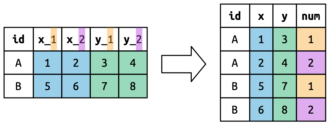

pivot_wider

pivot_wider() is the opposite of pivot_longer(), which you use if you have data for the same observation taking up multiple rows.

Here’s an example of data that we probably want to pivot wider (unless we want to plot each statistic in its own facet):

# A tibble: 6 × 3
  Group Statistic Value
  <chr> <chr>     <dbl>
1 A     Mean       1.28
2 A     Median     1   
3 A     SD         0.72
4 B     Mean       2.81
5 B     Median     2   
6 B     SD         1.33

A common cue to use pivot_wider() is having measurements of different quantities in the same column.

pivot_wider Example

wide_stats <- long_stats |> 
  pivot_wider(id_cols = Group,
              names_from = Statistic,
              values_from = Value)
wide_stats

8

id_cols is the column that uniquely identifies each row in the new dataset. Default is everything not in names_from and values_from.

9

names_from provides the names that will be used for the new columns

10

values_from provides the values that will be used to populate the cells of the new columns.

# A tibble: 2 × 4
  Group  Mean Median    SD
  <chr> <dbl>  <dbl> <dbl>
1 A      1.28      1  0.72
2 B      2.81      2  1.33

pivot_wider() also has a number of optional names_* and values_* arguments for more complicated transformations.

Nested Data

If there are multiple rows in the input that correspond to one cell in the output you’ll get a list-column. This means that you 1) need to fix something in your code/data because it shouldn’t be nested in this way or 2) need to use unnest_wider() or unnest_longer() in order to access this column of data. More on this here.

Useful Resources

Cheatsheets:

• readr
• dplyr
• tidyr

Introductory Book:

R for Data Science (2e) by Hadley Wickham, Mine Çetinkaya-Rundel, and Garrett Grolemund

CSSCR Consulting Services

CSSCR is a resource center for the social science departments¹ at the University of Washington.

As you continue to learn R feel free to drop by with any/all of your R coding questions. Below are our hours for the quarter:

The Center for Social Science Computation and Research
Consulting Hours for Fall 2024
	In-Person1	Virtual2
Monday	8am - 6pm	6 - 9pm
Tuesday	8am - 6pm	6 - 9pm
Wednesday	8am - 6pm	6 - 9pm
Thursday	8am - 6pm	6 - 9pm
Friday	8am - 5pm
1 Drop-in @ Savery 119 2 Online Via Zoom

1. Constituent member departments include The College of Education, The Department of Anthropology, The Department of Communication, The Department of Economics, The Department of Geography, The Department of Political Science, The Department of Psychology, The Department of Sociology, The Jackson School of International Studies, and The School of Social Work

Thanks!