| body | backpack |
|---|---|
| 120 | 26 |
| 187 | 30 |
| 109 | 26 |
| 103 | 24 |
| 131 | 29 |
| 165 | 35 |
| 158 | 31 |
| 116 | 28 |
Scatterplots and correlation
SOC 221 • Lecture 9
Monday, August 4, 2025
Correlation and Scatterplots
Scatterplot: A graph that uses points to simultaneously display the value on two variables for each case in the data
Allows us to picture the association between variables
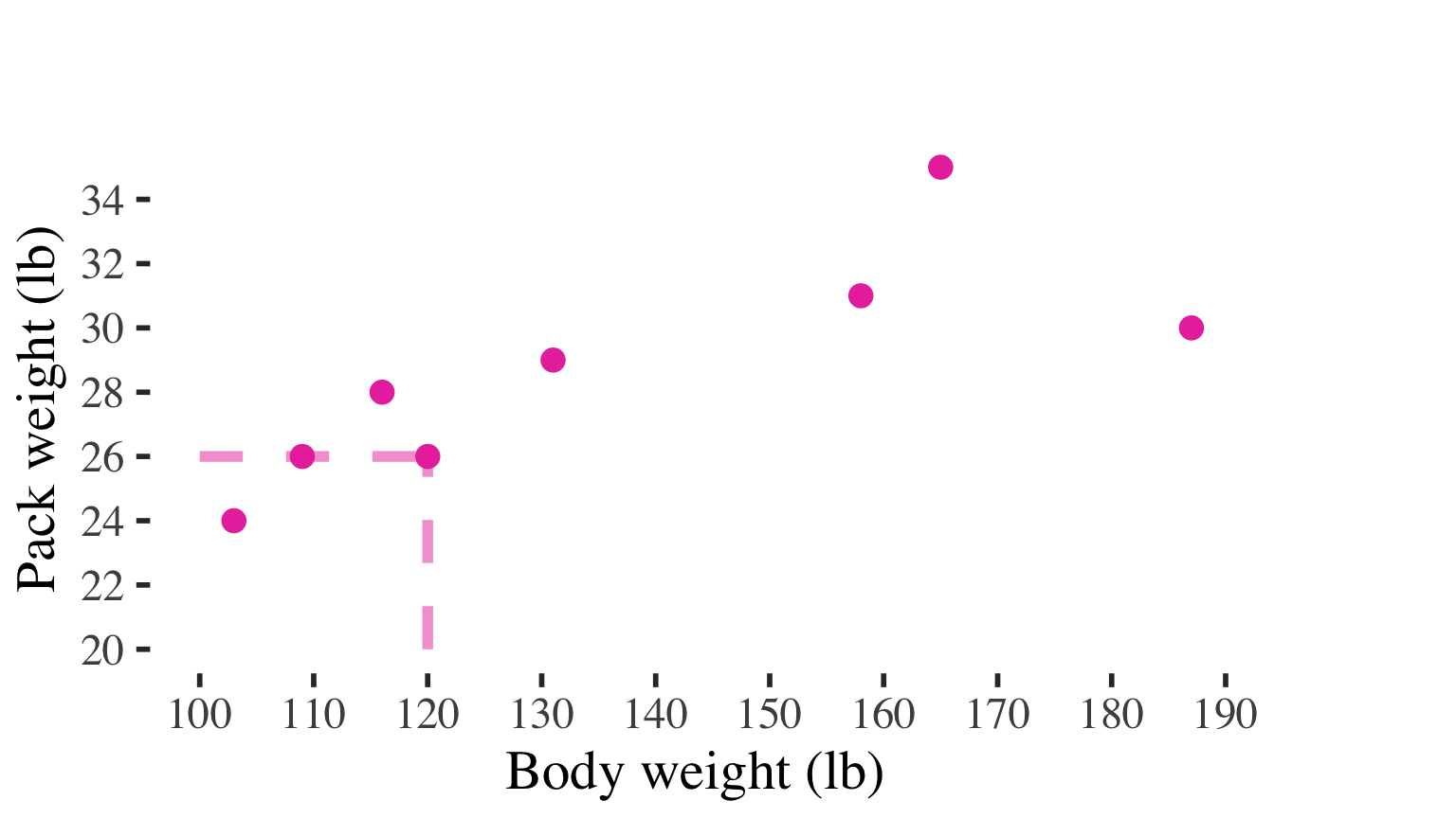
Example: Association between hiker weight and weight of backpack carried
Correlation and Scatterplots
Scatterplot: A graph that uses points to simultaneously display the value on two variables for each case in the data
Allows us to picture the association between variables
Example: Association between hiker weight and weight of backpack carried
| body | backpack |
|---|---|
| 120 | 26 |
| 187 | 30 |
| 109 | 26 |
| 103 | 24 |
| 131 | 29 |
| 165 | 35 |
| 158 | 31 |
| 116 | 28 |

X-axis (horizontal) displays all values in the IV
Y-axis (vertical) displays all values on the DV
Each dot represents a case, positioned along the X and Y axes
Correlation and Scatterplots
Scatterplot: A graph that uses points to simultaneously display the value on two variables for each case in the data
Allows us to picture the association between variables
Example: Association between hiker weight and weight of backpack carried
| body | backpack |
|---|---|
| 120 | 26 |
| 187 | 30 |
| 109 | 26 |
| 103 | 24 |
| 131 | 29 |
| 165 | 35 |
| 158 | 31 |
| 116 | 28 |
Can see the (positive) association
(high values on one variable tend to go with high values on the other)
Correlation and Regression
The two most common tool for measuring
associations between interval variables
CORRELATION
standardized summary of association between our variables
- does not depend on the units of the variables
- always 0 to |1.0|
- allows for comparison of associations between different pairs of variables
REGRESSION
characterizes the substantive effect of X on Y
- how much Y differs across different values of X
- conveyed in units of our specific independent and dependent variables
Both correlation and regression are based on a description of a line used to characterize data points in a scatterplot
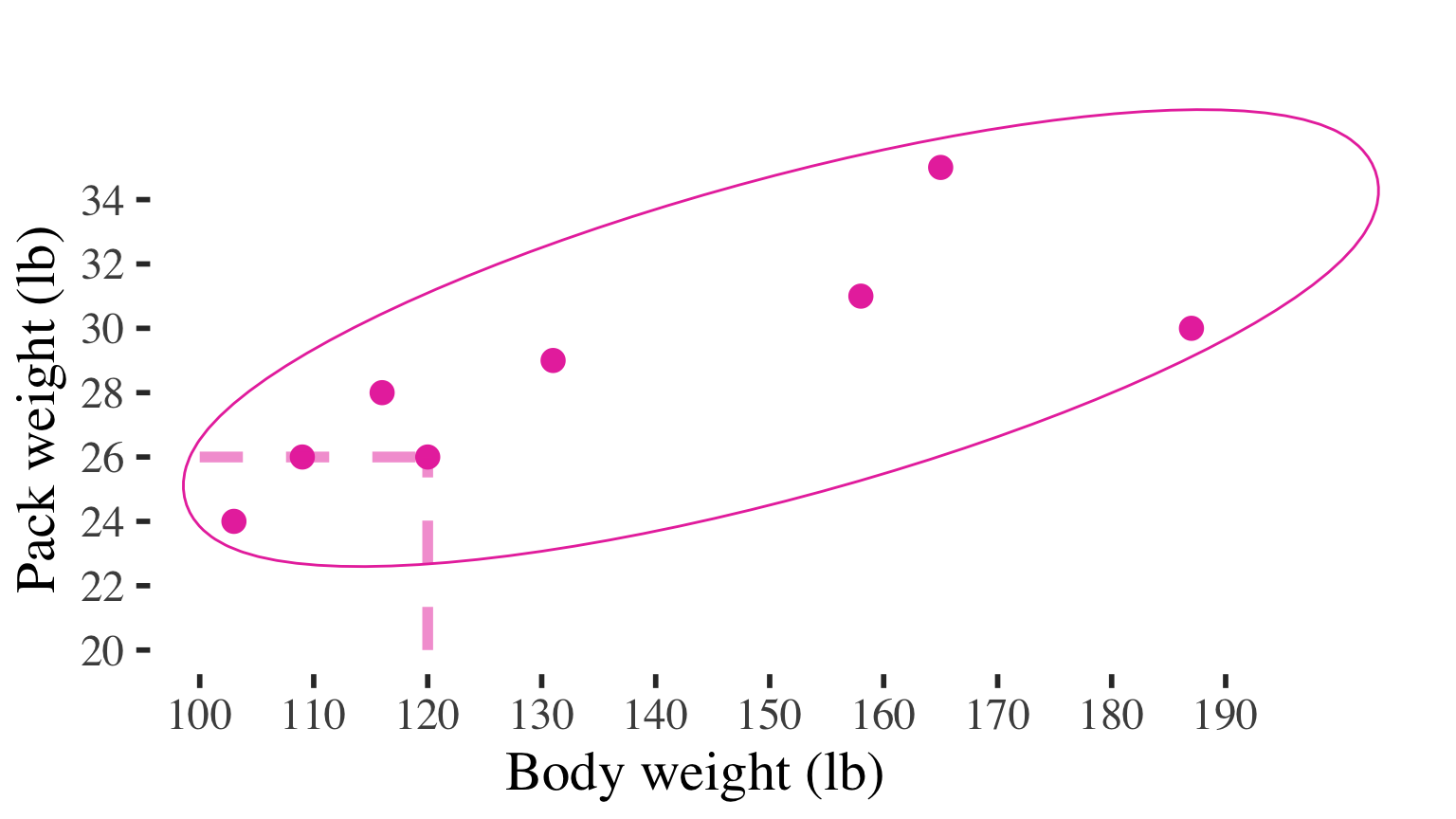
Scatterplots allow us to picture the association between variables
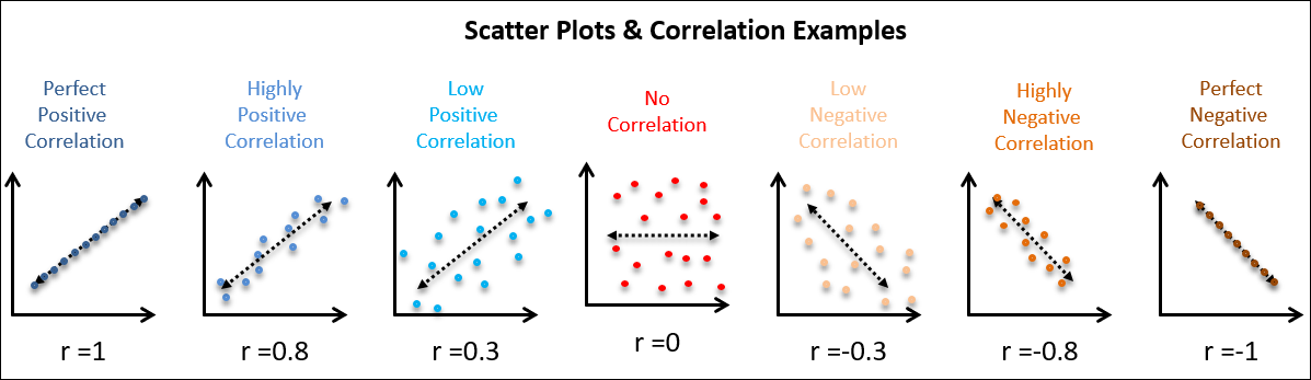
Stronger associations = more tightly clustered points
Weak associations have lots of conditional variation and not much difference in conditional distributions (distribution of the DV across values of the IV)
Strong associations have very little conditional variation and lots of difference in conditional distributions (distribution of the DV across values of the IV)
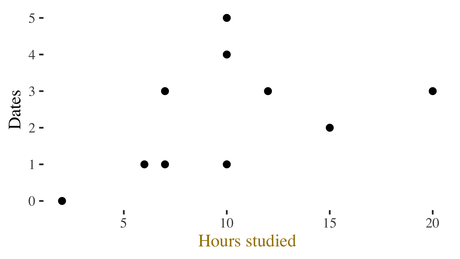
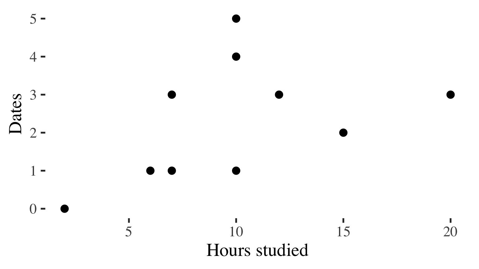
Making a scatterplot
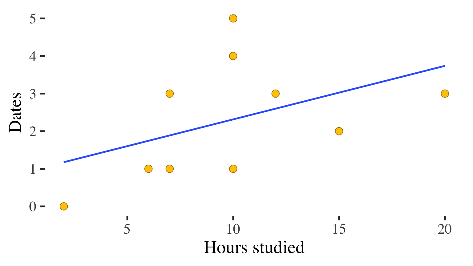
Example: Do people who study more have more or fewer dates?
| Hours studied | Dates |
|---|---|
| 10 | 1 |
| 15 | 2 |
| 10 | 5 |
| 6 | 1 |
| 2 | 0 |
| 7 | 3 |
| 10 | 4 |
| 12 | 3 |
| 7 | 1 |
| 20 | 3 |

Making a scatterplot
Example: Do people who study more have more or fewer dates?
| Hours studied | Dates |
|---|---|
| 10 | 1 |
| 15 | 2 |
| 10 | 5 |
| 6 | 1 |
| 2 | 0 |
| 7 | 3 |
| 10 | 4 |
| 12 | 3 |
| 7 | 1 |
| 20 | 3 |
Making a scatterplot
Example: Do people who study more have more or fewer dates?
| Hours studied | Dates |
|---|---|
| 10 | 1 |
| 15 | 2 |
| 10 | 5 |
| 6 | 1 |
| 2 | 0 |
| 7 | 3 |
| 10 | 4 |
| 12 | 3 |
| 7 | 1 |
| 20 | 3 |
Making a scatterplot
Example: Do people who study more have more or fewer dates?
| Hours studied | Dates |
|---|---|
| 10 | 1 |
| 15 | 2 |
| 10 | 5 |
| 6 | 1 |
| 2 | 0 |
| 7 | 3 |
| 10 | 4 |
| 12 | 3 |
| 7 | 1 |
| 20 | 3 |
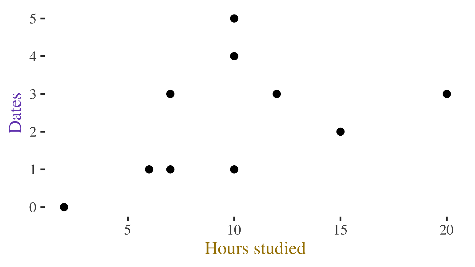
Can see the association
Correlation coefficient allows us to quantify/summarize that association
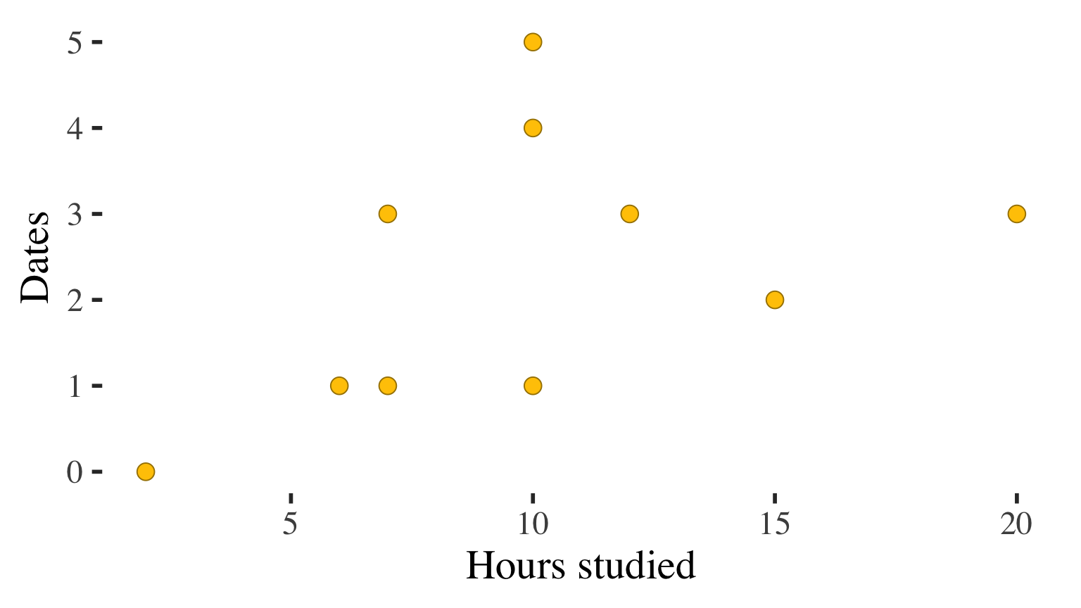
Association between hours studied and number of dates
| Hours studied | Dates |
|---|---|
| 10 | 1 |
| 15 | 2 |
| 10 | 5 |
| 6 | 1 |
| 2 | 0 |
| 7 | 3 |
| 10 | 4 |
| 12 | 3 |
| 7 | 1 |
| 20 | 3 |
Description of the association?
Correlation \(r = 0.456\)
Positive, moderate association
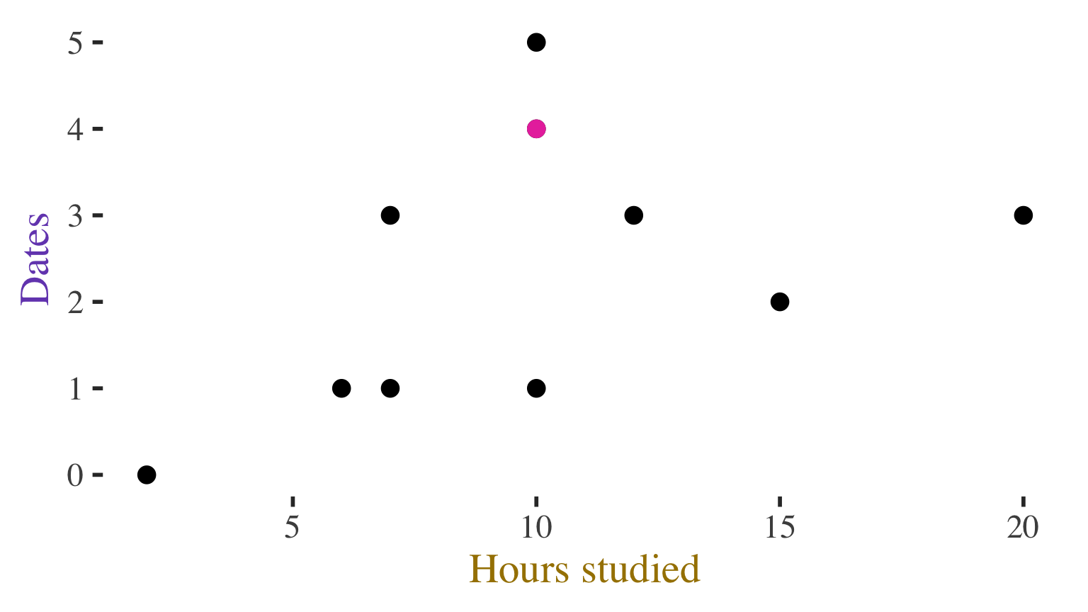
Association between hours studied and number of dates
| Hours studied | Dates |
|---|---|
| 10 | 1 |
| 15 | 2 |
| 10 | 5 |
| 6 | 1 |
| 2 | 0 |
| 7 | 3 |
| 10 | 4 |
| 12 | 3 |
| 7 | 1 |
| 20 | 3 |
Description of the association?
Correlation \(r = 0.456\)
Positive, moderate association
This is the DIRECTION and STRENGTH of
the association in the SAMPLE
Want to know whether there is an association
in the POPULATION (i.e., whether the
observed association is statistically significant)
Need a hypothesis test…
Hypothesis test for correlation
- Check assumptions
- Random sample, variables roughly normally distributed in the population, linear relationship, homoscedasticity
Similar error of prediction (similar spread around the line) at all values of X

Association between hours studied and number of dates
\(r = 0.456\)
Positive, moderate association in the sample
1. Check assumptions
- Random sample?
- Variables roughly normally distributed in the population?
- check sample distributions for a clue
- Linear relationship
- Check scatterplot
- Homoscedasticity
- Similar error of prediction (similar spread around the line) at all values of X
- Check scatterplot