Estimation: confidence intervals
for means and proportions
SOC 221 • Lecture 6
Wednesday, July 16, 2025
Estimation: confidence intervals for means
Using these tools for inference
Example: Want to know how much UW students study on average
\(\bar{X}\) —INFERENCE–> \(\mu_x\)
Sample statistic: The characteristic of the sample that we actually observe (i.e. the mean study time of a SAMPLE of UW students)
For example: draw a random sample of 100 students and observe \(\bar{X} = 14.5\)
Population parameter: The characteristic of the population that we are interested in knowing (i.e. the mean study time of all UW students)
Our goal: Estimate the unknown population parameter \(\mu_x = ?\)
Sampling distribution
Sampling Distribution
A theoretical probability distribution of all possible sample values for the statistic in which we are interested.
Key tool for inferential statistics
Allows us to think about how our one single sample result relates to all possible sample results and, by extension, the population we are interested in drawing inferences about.
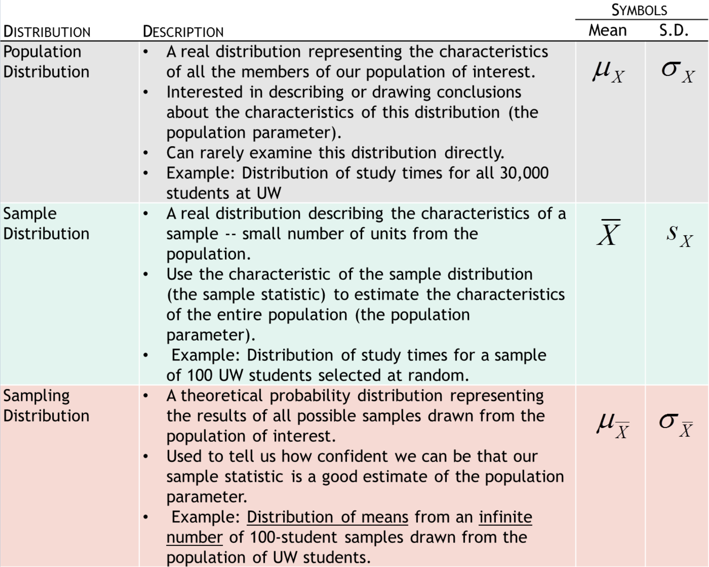
Three types of distributions

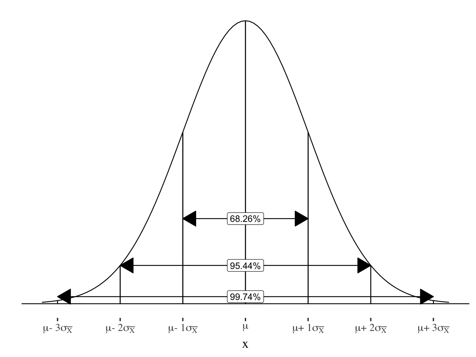
Implication of central limit theorem
- Central limit theorem tells us that if the size of our random sample is large enough, we can assume that the sampling distribution of all such possible samples is:
- Normally distributed
- Mean: \(\mu_\bar{X}\) \(= \mu_X\)
- Standard Error = \(\sigma_\bar{X}\) \(= \frac{\sigma}{\sqrt{n}}\)
Standard error:
The the standard deviation
in the sampling distribution
(in this case, of all
possible sample means)

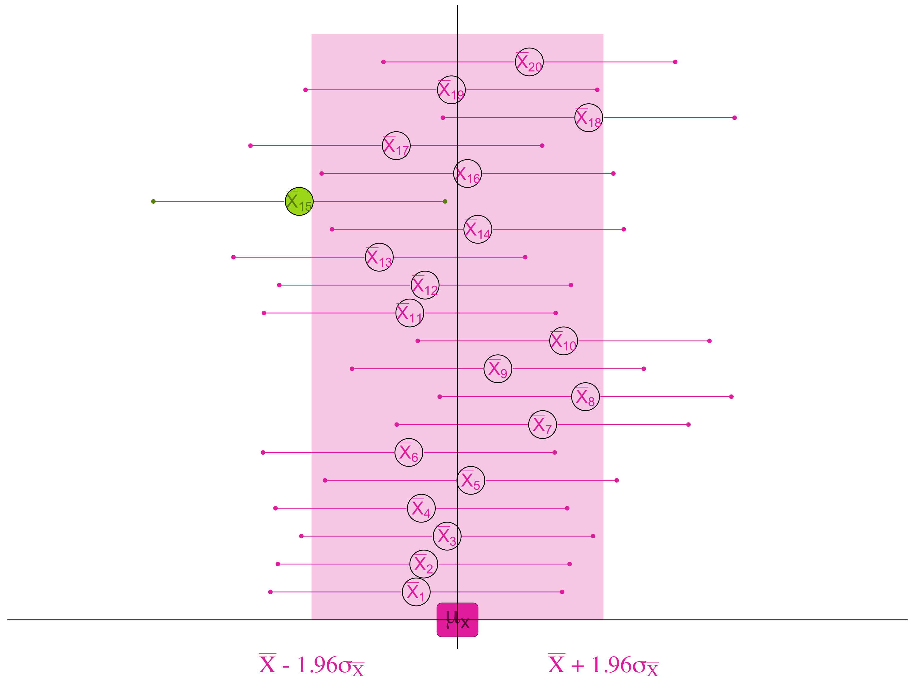
If, 95% of the samples are within 1.96 standard errors of the true population mean . . .
. . . then for 95 samples out of 100, we will find the true population mean if we look within 1.96 standard errors of the sample mean.
Confidence intervals
The BIG IDEA:
- The sampling distribution and CLT tells us how close to the population mean (\(\mu\)) the sample mean (\(\bar{X}\)) is likely to be
- We can use this knowledge to figure out how close to the one sample mean (\(\bar{X}\)) that we observe the true population mean (\(\mu\)) is likely to be
- Build a confidence interval around our sample statistic (mean) to define the range in which we think the population parameter can be found…
- … and quantify how likely it is that we are right
Using these tools for inference
Example: Want to know how much UW students study on average
\(\bar{X}\) —INFERENCE–> \(\mu_x\)
Sample statistic: The characteristic of the sample that we actually observe (i.e. the mean study time of a SAMPLE of UW students)
For example: draw a random sample of 100 students and observe \(\bar{X} = 14.5\)
Population parameter: The characteristic of the population that we are interested in knowing (i.e. the mean study time of all UW students)
Our goal: Estimate the unknown population parameter \(\mu_x = ?\)
Confidence intervals
\[ \bar{X} \]
Create a range of scores, centered on the sample mean, in which we think the population mean is likely to be located
Building a margin of error around our sample mean
Confidence interval:
\(\text{sample statistic} \pm \text{margin of error}\)
⬅️
All confidence intervals take this form
Confidence intervals
\[ \bar{X} \]
Confidence interval:
\(\text{sample statistic} \pm \text{margin of error}\)
\(\text{sample statistic} \pm z \text{(standard error)}\)
\(\bar{X} \pm z(\sigma_{\bar{X}})\)
Calculating confidence intervals
Step 1: Decide on a confidence level and corresponding z-score
Step 2: Calculate the standard error
Step 3: Calculate the margin of error
Step 4: Calculate the confidence interval
Step 5: Interpret the results
Calculating confidence intervals
Step 1: Decide on a confidence level and corresponding z-score
Step 2: Calculate the standard error
Step 3: Calculate the margin of error
Step 4: Calculate the confidence interval
Step 5: Interpret the results
Step 1: Decide on a confidence level and corresponding z-score
- Confidence level (C) refers to the level of confidence that you will have in your inference
- Example: For a 95% confidence interval, you will be able to say that you are 95% confident that the true population mean falls within the interval
- More accurately, the probability that the confidence interval contains the actual population parameter
- 95% of all possible samples of a given size from this population will result in an interval that captures the unknown parameter.
- Most common: 90%, 95%, and 99%
| 50% | 60% | 70% | 80% | 90% | 95% | 96% | 98% | 99% | 99.5% | 99.9% | |
|---|---|---|---|---|---|---|---|---|---|---|---|
| Z* | 0.674 | 0.841 | 1.036 | 1.282 | 1.645 | 1.960 | 2.054 | 2.326 | 2.576 | 2.807 | 3.291 |
To create a \(95\%\) confidence interval, go out \(1.96\) standard errors on each side of the sample mean
Calculating confidence intervals
Step 1: Decide on a confidence level and corresponding z-score
Step 2: Calculate the standard error
Step 3: Calculate the margin of error
Step 4: Calculate the confidence interval
Step 5: Interpret the results
Step 2: Calculate the standard error
- Standard error = standard deviation of the sampling distribution
- Central Limit Theorem tells us:
\[ \sigma_{\bar{X}} = \frac{\sigma}{\sqrt{n}} \]
Example: Say you know that your sample of 100 people comes from a population with a standard deviation of 8.0
\[ \sigma_{\bar{X}} = \frac{\sigma}{\sqrt{n}} = \frac{8.0}{\sqrt{100}} = 0.8 \]
Calculating confidence intervals
Step 1: Decide on a confidence level and corresponding z-score
Step 2: Calculate the standard error
Step 3: Calculate the margin of error
Step 4: Calculate the confidence interval
Step 5: Interpret the results
Step 3: Calculate the margin of error
Margin of error = how far out on each side of the sample mean we need to go to define our confidence interval
\[ \text{margin of error} = z(\sigma_{\bar{X}}) = z(\frac{\sigma}{\sqrt{n}}) \]
Margin of error for our example:
\[ z(\frac{\sigma}{\sqrt{n}}) = (1.96)(0.8)= 1.57 \]
Interpretation:
Need to go out 1.57 hours on each side of the sample mean to be 95% confident that we have captured the true population mean.
Calculating confidence intervals
Step 1: Decide on a confidence level and corresponding z-score
Step 2: Calculate the standard error
Step 3: Calculate the margin of error
Step 4: Calculate the confidence interval
Step 5: Interpret the results
Step 4: Calculate the confidence interval
- Add and then subtract the margin of error from the sample mean to get the upper and lower bounds of your confidence interval
Confidence interval:
\(\text{sample statistic} \pm \text{margin of error}\)
Example:
\[ 14.5 + 1.57 = 16.07 \]
\[ 14.5 - 1.57 = 12.93 \]
\(95\%\) confidence interval:
\(12.93\) to \(16.07\) hours
Calculating confidence intervals
Step 1: Decide on a confidence level and corresponding z-score
Step 2: Calculate the standard error
Step 3: Calculate the margin of error
Step 4: Calculate the confidence interval
Step 5: Interpret the results
Step 5: Interpret the results
- A complete interpretation of a confidence interval has three components
- Level of confidence (usually 90%, 95%, 99%)
- Reference to the population parameter being estimated
- The interval of values (or at least the sample statistic and margin of error)
Example:
\(95\%\) confidence interval:
\(12.93\) to \(16.07\) hours
We are \(95\%\) confident that the true average number of hours studied for the population of UW students is between \(12.93\) to \(16.07\) hours
Practice
Mean texts per hour
- Suppose that the number of text messages sent per hour by the population of teenagers has a standard deviation of 3
- You take a random sample of 144 teenagers and find that the mean number of text messages per hour is 4.5
- Calculate a 90% confidence interval to estimate the average number of text messages per hour in the population
- Step 1: Use z = 1.645
- Step 2: Calculate standard error \[ \sigma_{\bar{X}} = \frac{\sigma}{\sqrt{n}} = \frac{3.0}{\sqrt{144}} = 0.25 \]
- Step 3: Calculate the margin of error \[ z(\frac{\sigma}{\sqrt{n}}) = (1.645)(0.25)= 0.411 \]
| 50% | 60% | 70% | 80% | 90% | 95% | 96% | 98% | 99% | 99.5% | 99.9% | |
|---|---|---|---|---|---|---|---|---|---|---|---|
| Z* | 0.674 | 0.841 | 1.036 | 1.282 | 1.645 | 1.960 | 2.054 | 2.326 | 2.576 | 2.807 | 3.291 |
\(\text{sample statistic} \pm \text{margin of error}\)
Practice
Mean texts per hour
\(\text{sample statistic} \pm \text{margin of error}\)
- Suppose that the number of text messages sent per hour by the population of teenagers has a standard deviation of 3
- You take a random sample of 144 teenagers and find that the mean number of text messages per hour is 4.5
- Calculate a 90% confidence interval to estimate the average number of text messages per hour in the population
- Step 4: Calculate the confidence interval \[ 4.5 + 0.411 = 4.911 \] \[ 4.5 - 0.411 = 4.089 \]
\(90\%\) confidence interval:
\(4.09\) to \(4.91\) hours
| 50% | 60% | 70% | 80% | 90% | 95% | 96% | 98% | 99% | 99.5% | 99.9% | |
|---|---|---|---|---|---|---|---|---|---|---|---|
| Z* | 0.674 | 0.841 | 1.036 | 1.282 | 1.645 | 1.960 | 2.054 | 2.326 | 2.576 | 2.807 | 3.291 |
Practice
Mean texts per hour
\(\text{sample statistic} \pm \text{margin of error}\)
- Suppose that the number of text messages sent per hour by the population of teenagers has a standard deviation of 3
- You take a random sample of 144 teenagers and find that the mean number of text messages per hour is 4.5
- Calculate a 90% confidence interval to estimate the average number of text messages per hour in the population
- Step 5: Interpret the results
We are 90% confident that the average number of texts sent per hour for the population of teenagers is between 4.09 and 4.91
| 50% | 60% | 70% | 80% | 90% | 95% | 96% | 98% | 99% | 99.5% | 99.9% | |
|---|---|---|---|---|---|---|---|---|---|---|---|
| Z* | 0.674 | 0.841 | 1.036 | 1.282 | 1.645 | 1.960 | 2.054 | 2.326 | 2.576 | 2.807 | 3.291 |
Factors affecting precision (width) of the confidence interval
- Which confidence interval would you prefer?
- Average study time of UW students is between 10.5 and 18.5 hours
OR - Average study time of UW students is between 14.25 and 14.75 hours
- Average study time of UW students is between 10.5 and 18.5 hours
All else being equal, the second one is preferable because it is more precise
(narrower, with smaller margin of error)
Factors affecting precision (width) of the confidence interval
\[ \text{margin of error} = z(\frac{\sigma}{\sqrt{n}}) \]
- Confidence level
- Trade-off: higher confidence = lower precision (higher margin of error)
| 50% | 60% | 70% | 80% | 90% | 95% | 96% | 98% | 99% | 99.5% | 99.9% | |
|---|---|---|---|---|---|---|---|---|---|---|---|
| Z* | 0.674 | 0.841 | 1.036 | 1.282 | 1.645 | 1.960 | 2.054 | 2.326 | 2.576 | 2.807 | 3.291 |
- Sample size
- Larger sample = smaller standard error = greater precision (lower margin of error)
- Level of variation in the population
- More variation in population = more variation in possible sample results = larger standard error = bigger margin of error
Break!
Estimation: confidence intervals for proportions
Estimating Population Proportions (or percentages)
Goal:
- Use the sample proportion (\(\widehat{p}\)) to construct a confidence interval in which we believe the true population proportion (\(P\))1 is located
Example:
- Want to know the proportion of UW students who are employed during the school year
- Population proportion, \(P\), is not observable
- Use sample information to estimate \(P\)
- \(n = 200\)
- Sample proportion, \(\hat{p} = 0.42\)
Confidence intervals
\[ \widehat{p} \]
Create our 95% confidence interval by going 1.96 standard errors on each side of the sample proportion
Building a margin of error around our sample proportion
Confidence interval:
\(\text{sample statistic} \pm \text{margin of error}\)
Calculating confidence intervals
Step 1: Decide on a confidence level and corresponding z-score
Step 2: Calculate the standard error
Step 3: Calculate the margin of error
Step 4: Calculate the confidence interval
Step 5: Interpret the results
Step 1: Decide on a confidence level and corresponding z-score
- Confidence level (C) refers to the level of confidence that you will have in your inference
- Example: For a 95% confidence interval, you will be able to say that you are 95% confident that the true population mean falls within the interval
- More accurately, the probability that the confidence interval contains the actual population parameter
- 95% of all possible samples of a given size from this population will result in an interval that captures the unknown parameter.
- Most common: 90%, 95%, and 99%
| 50% | 60% | 70% | 80% | 90% | 95% | 96% | 98% | 99% | 99.5% | 99.9% | |
|---|---|---|---|---|---|---|---|---|---|---|---|
| Z* | 0.674 | 0.841 | 1.036 | 1.282 | 1.645 | 1.960 | 2.054 | 2.326 | 2.576 | 2.807 | 3.291 |
To create a \(95\%\) confidence interval, go out \(1.96\) standard errors on each side of the sample mean
Step 2: Calculate the standard error
- Standard error = standard deviation of the sampling distribution
- Central Limit Theorem tells us:
\[ \sigma_{\widehat{p}} = \sqrt{\frac{\widehat{p}(1-\widehat{p})}{n}} \]
where \(\widehat{p}\) = sample proportion
\(n\) = sample size
Example: With sample size of 200 and sample proportion of 0.42
\[ \sigma_{\widehat{p}} = \sqrt{\frac{\widehat{p}(1-\widehat{p})}{n}} = \sqrt{\frac{0.42(1-0.42)}{200}} = 0.035 \]
Step 3: Calculate the margin of error
Margin of error = how far out on each side of the sample mean we need to go to define our confidence interval
\[ \text{margin of error} = z(\sigma_{\widehat{p}}) = z(\sqrt{\frac{\widehat{p}(1-\widehat{p})}{n}}) \]
Margin of error for our example:
\[ z(\sqrt{\frac{\widehat{p}(1-\widehat{p})}{n}}) = (1.96)(0.035) = 0.069 \]
Interpretation:
Need to go out 0.069 in each direction of the sample proportion to be 95% confident that we have captured the true population proportion.
Step 4: Calculate the confidence interval
- Add and then subtract the margin of error from the sample mean to get the upper and lower bounds of your confidence interval
Confidence interval:
\(\text{sample statistic} \pm \text{margin of error}\)
Example:
\[ 0.42 + 0.069 = 0.489 \]
\[ 0.42 - 0.069 = 0.351 \]
\(95\%\) confidence interval:
\(0.351\) to \(0.489\)
Step 5: Interpret the results
- A complete interpretation of a confidence interval has three components
- Level of confidence (usually 90%, 95%, 99%)
- Reference to the population parameter being estimated
- The interval of values (or at least the sample statistic and margin of error)
Example:
\(95\%\) confidence interval:
\(0.351\) to \(0.489\)
We are \(95\%\) confident that between \(35.1\%\) and \(48.9\%\) of the population of students are employed during the school year.
Practice
Household Purchasing Decisions
Suppose a marketing company did a survey of 200 randomly selected households and found that in 120 of them, the woman made the majority of the purchasing decisions. We are interested in the population proportion of households where women make the majority of the purchasing decisions.
- Construct a 95% confidence interval for the population proportion of households where the women make the majority of the purchasing decisions.
- List two difficulties the company might have in obtaining random results, if this survey were done by email.
Practice
Construct a 95% confidence interval for the population proportion of households where the women make the majority of the purchasing decisions.
Identify the sample proportion
\[ \hat{p} = \frac{120}{200} = 0.60 \]
This is our sample proportion — the best estimate of the true population proportion.
Compute the standard error
\[ \sigma_{\widehat{p}} = \sqrt{\frac{\widehat{p}(1-\widehat{p})}{n}} = \sqrt{\frac{0.60(1 - 0.60)}{200}} = \sqrt{\frac{0.60 \cdot 0.40}{200}} = \sqrt{\frac{0.24}{200}} = \sqrt{0.0012} \approx 0.0346 \]
Compute the margin of error
\[ \text{margin of error} = z(\sigma_{\widehat{p}}) = 1.96(0.0346) \approx 0.0678 \]
Compute the confidence interval
\[ \text{CI} = 0.60 \pm 0.0678 = (0.5322, 0.6678) \]
Practice
Construct a 95% confidence interval for the population proportion of households where the women make the majority of the purchasing decisions.
Interpretation
We are 95% confident that between 53.2% and 66.8% of the population of all households have women making the majority of purchasing decisions.
Practice
List two difficulties the company might have in obtaining random results, if this survey were done by email.
- Selection/Coverage Bias: Not all households have equal access to or use email regularly. Households with older adults, that are low-income, or have limited internet access may be underrepresented, making the sample non-random.
- Non-response Bias: People who ignore survey emails may differ in important ways from those who respond. For example, more engaged, time-rich individuals may reply, skewing results.
- Sampling Frame Challenges: How will the study create the sampling frame needed to randomly sample households using emails addresses? Many people have multiple email addresses - how will that be accounted for? How will selection within households be done? Given the complexity of conducting an unbiased sample using email addresses, the resulting sample is likely going to be collected using non-probabalistic methods (i.e. convenience sampling) which is not random