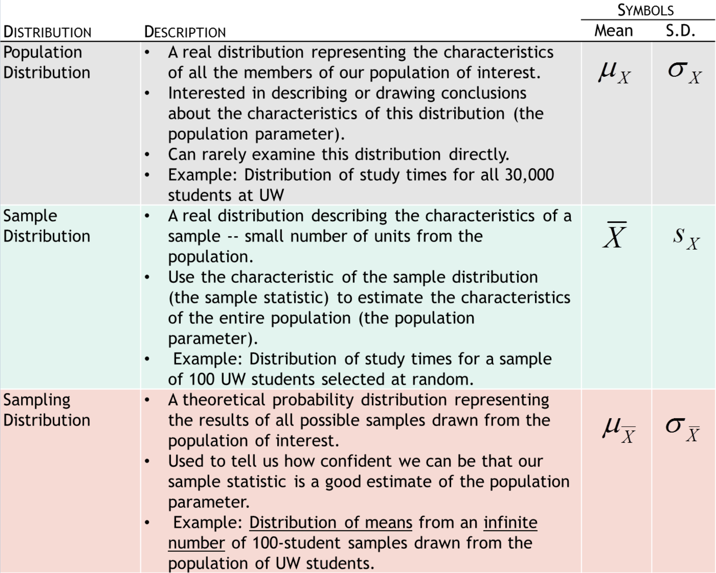
Sampling distributions,
Central limit theorem,
& the Logic of inference

SOC 221 • Lecture 5

Victoria Sass

Monday, July 7, 2025

Sampling distributions

Descriptive –> Inferential statistics

Where are we?

• So far: Worked on descriptive statistics – tools to describe distributions
• NEXT: Building the tools for inferential statistics

• Example: Want to know about the average study time for the population of UW students.
• NEXT: Building the tools for inferential statistics

Inferential statistics
Statistical procedures used
to draw conclusions
(or inferences) about
a population based on
data drawn from a sample

\(\bar{X}\) —INFERENCE–> \(\mu_x\)

Descriptive –> Inferential statistics

Where are we?

• So far: Worked on descriptive statistics – tools to describe distributions
• NEXT: Building the tools for inferential statistics

• Example: Want to know about the average study time for the population of UW students.
• NEXT: Building the tools for inferential statistics

Inferential statistics
Statistical procedures used
to draw conclusions
(or inferences) about
a population based on
data drawn from a sample

\(\bar{X}\) —INFERENCE–> \(\mu_x\)

Population parameter: The characteristic of the population that we are interested in knowing (i.e. the mean study time of all UW students)

Sample statistic: The characteristic of the sample that we actually observe (i.e. the mean study time of a SAMPLE of UW students)

The challenge of making inferences

Drawing inferences entails uncertainty

Even with a good sample, the sample is likely to differ from the population (sample statistic is likely to be different from our population parameter, just by chance)

Challenge

Assessing the risk of being wrong (being way off) in making an inference from observed sample statistics to unknown population parameters.

Key questions

1. How often would this procedure (drawing a sample, inferring about the population) give us something close to the correct answer if I used it over and over?
   or
2. What is the probability that the inference I draw from one sample is wrong (way off from the population characteristic of interest)?

Using these tools for inference

Example: Want to know how much UW students study on average

\(\bar{X}\) —INFERENCE–> \(\mu_x\)

Sample statistic: The characteristic of the sample that we actually observe (i.e. the mean study time of a SAMPLE of UW students)

For example: draw a random sample of 100 students and observe \(\bar{X} = 14.5\)

Population parameter: The characteristic of the population that we are interested in knowing (i.e. the mean study time of all UW students)

Our goal: Estimate the unknown population parameter \(\mu_x = ?\)

Estimating Population Parameters: TWO OPTIONS

One option: Just assume that the population mean is equal to the sample mean

\[ \mu_x = \bar{X} = 14.5 \]

• Called a point estimate

Potential problems with this strategy?

• Very likely to be wrong!
  • Even with a random sample, the sample statistic is like to miss the true population parameter by at least a little
    • Reflects chance sampling error
  • In reality:

\[ \mu_x \neq \bar{X} \]

SAMPLING ERROR
The difference
between a sample
statistic used to
estimate a population
parameter and the
actual (but unknown)
value of the
population
parameter.

Estimating Population Parameters: TWO OPTIONS

Better option: Create a CONFIDENCE INTERVAL

\[ \bar{X} \]

CONFIDENCE INTERVAL
A range of scores, centered on the sample mean, in which we think the population mean is likely to be located.

Building a margin of error around our sample mean

Estimating Population Parameters: TWO OPTIONS

Better option: Create a CONFIDENCE INTERVAL

\[ \bar{X} \]

Confidence intervals are defined by the Confidence Level (our certainty that the confidence interval will contain the true population parameter)

With a 95% confidence interval, we are 95% sure that the interval we construct contains the true population parameter we are interested in.

Over the long run, there is a probability of .99 that the actual population parameter falls within a 99% confidence interval that we construct

Estimating Population Parameters: TWO OPTIONS

Better option: Create a CONFIDENCE INTERVAL

\[ \bar{X} \]

CONFIDENCE INTERVAL
A range of scores, centered on the sample mean, in which we think the population mean is likely to be located.

Q: What is the ADVANTAGE of a confidence interval over a point estimate?

A: We are less likely to be wrong, and we can quantify the risk of being wrong.

Sampling distribution

Sampling Distribution
A theoretical probability distribution of all possible sample values for the statistic in which we are interested.

Key tool for inferential statistics

Allows us to think about how our one single sample result relates to all possible sample results and, by extension, the population we are interested in drawing inferences about.

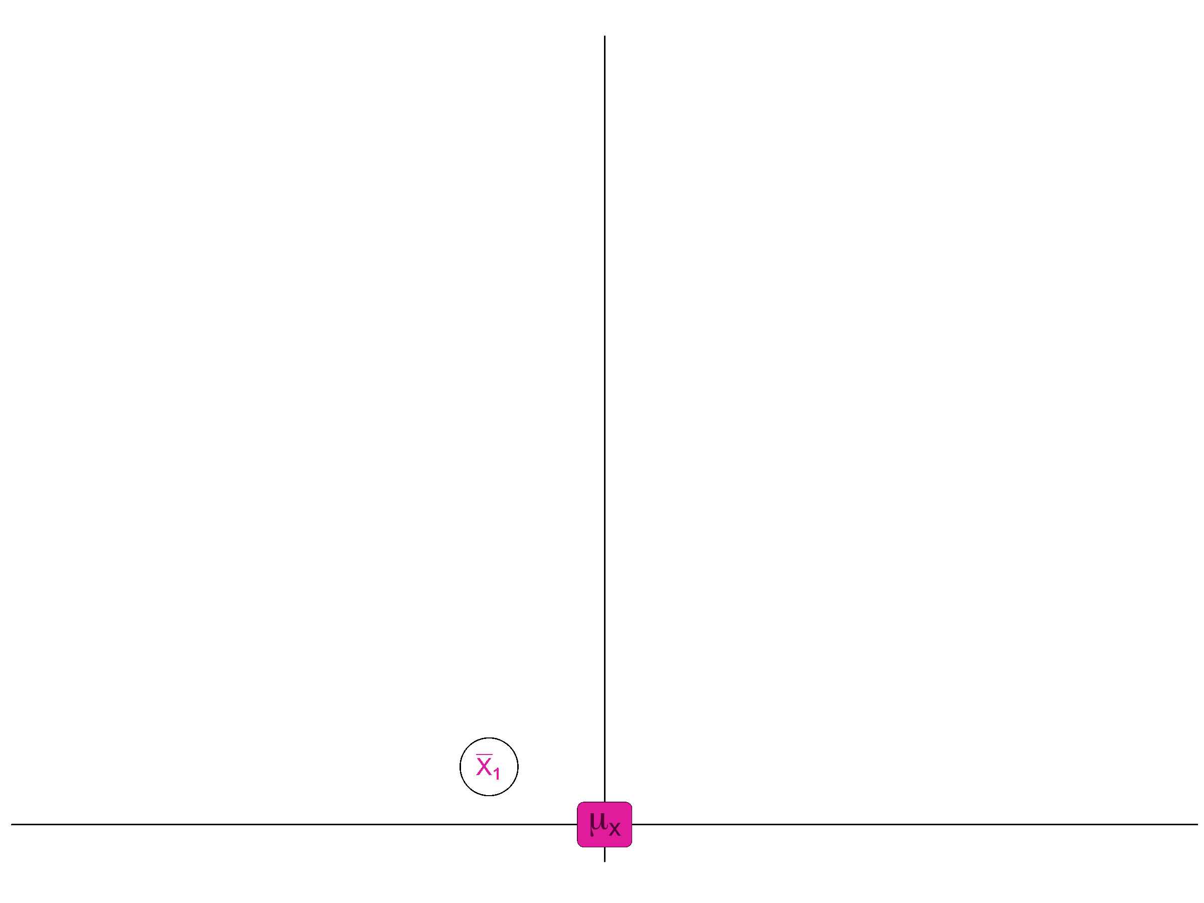
Imagine drawing ONE sample from the population and calculating the sample mean

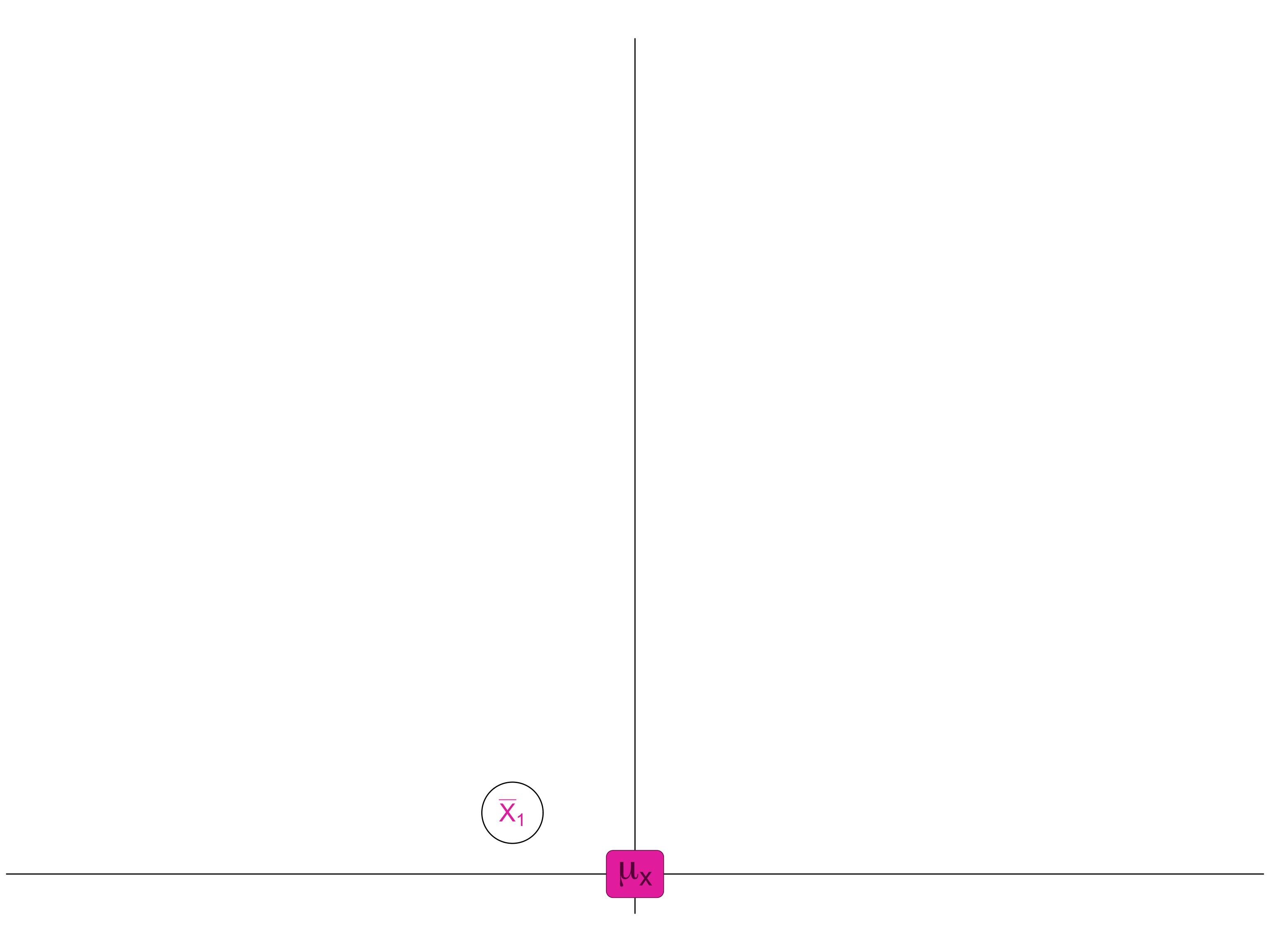
Imagine drawing ONE sample from the population and calculating the sample mean

Just by chance, our sample mean may be a little different than the true population mean.

Distance between the sample mean and the actual population mean reflects random sampling error

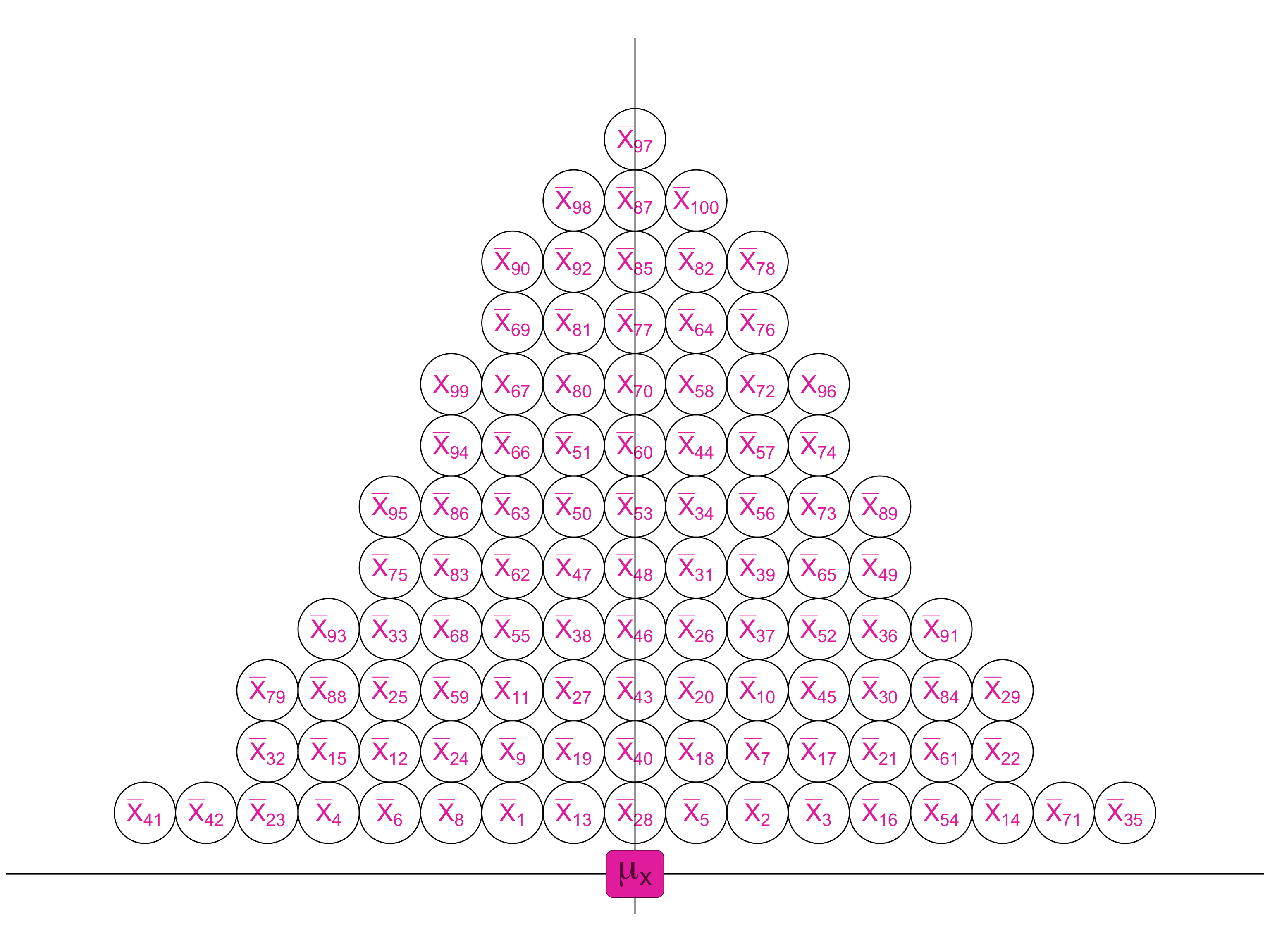
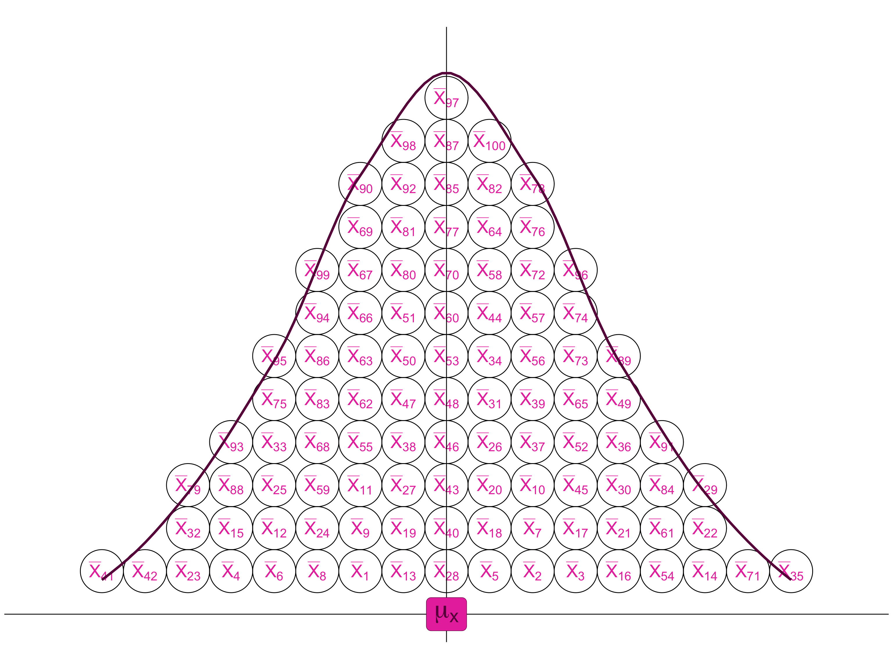
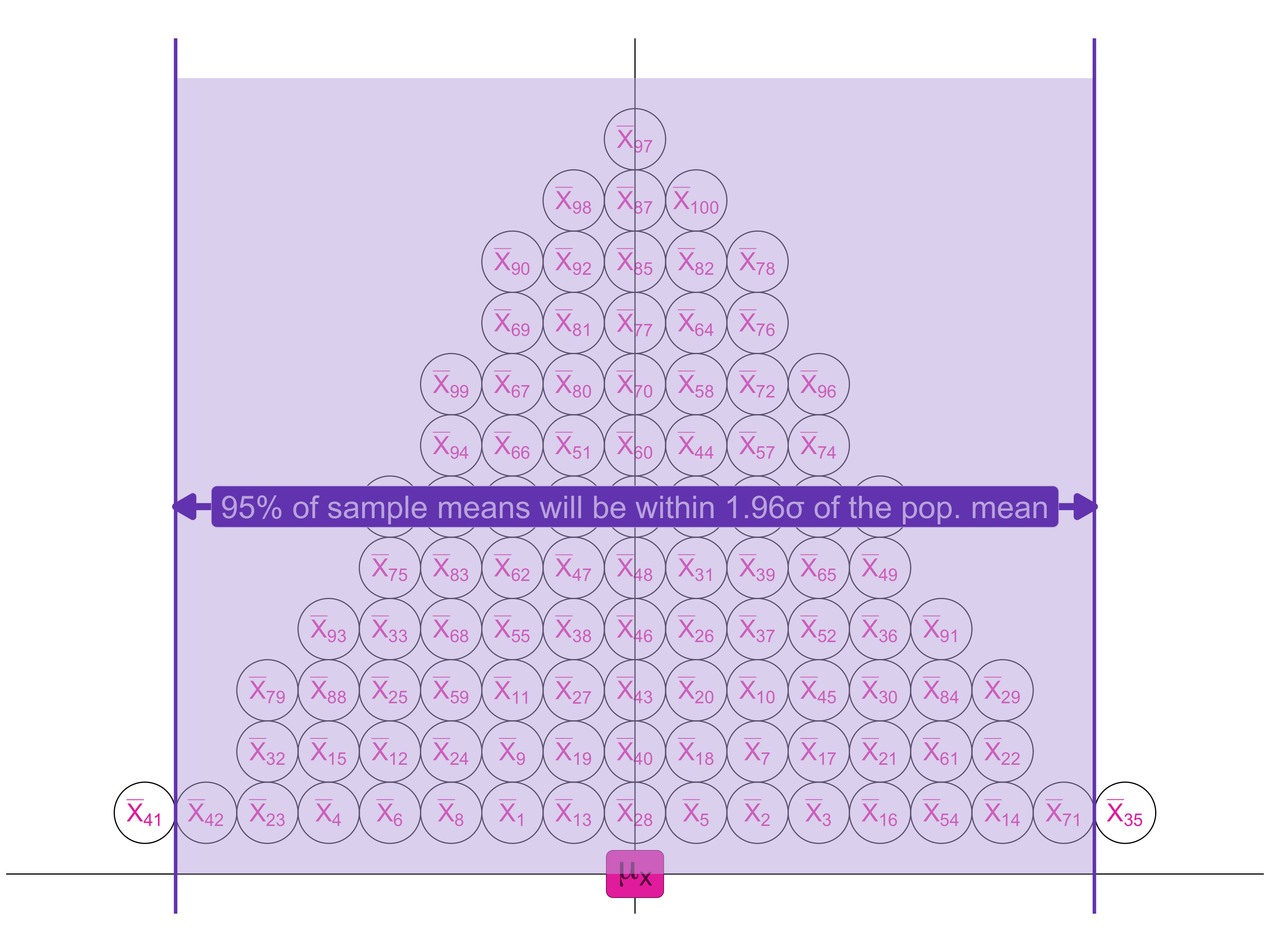
Now imagine drawing LOTS of independent samples and calculating the mean of X for each one.

Interesting features of the
sampling distribution
(when certain conditions are met):
• Normal distribution
• Mean of the sampling distribution is equal to the population mean

This produces a SAMPLING DISTRIBUTION of sample means

So can use what we know about the normal distribution to think about the location of sample means relative to the population mean.

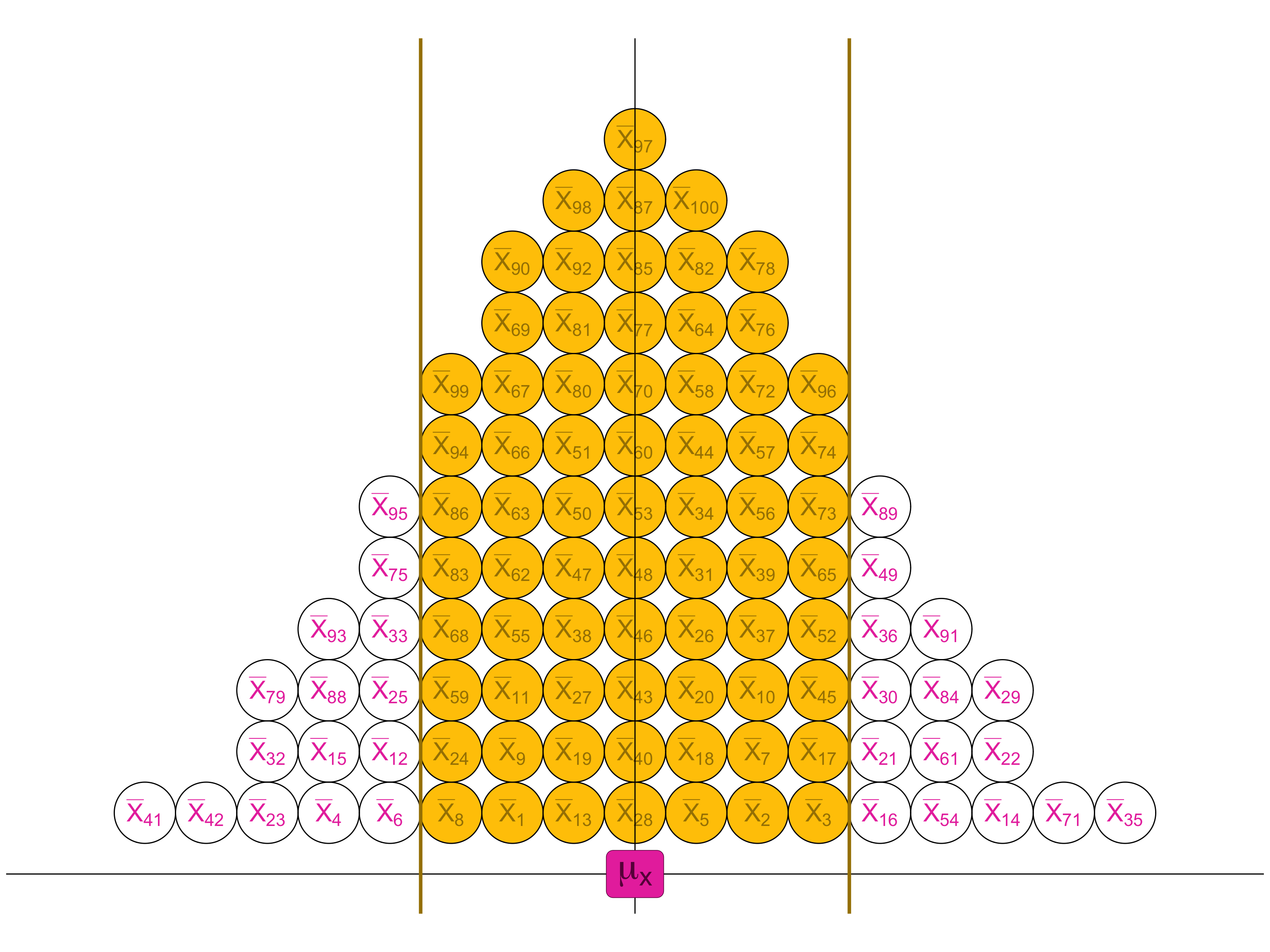
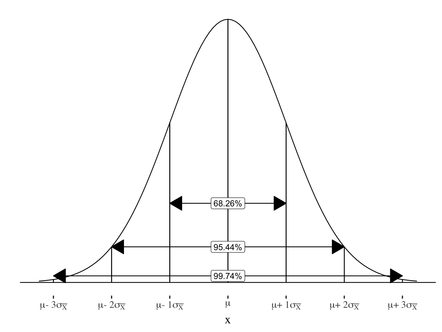
68.26% of samples will be within 1 \(\sigma\) of the pop. mean

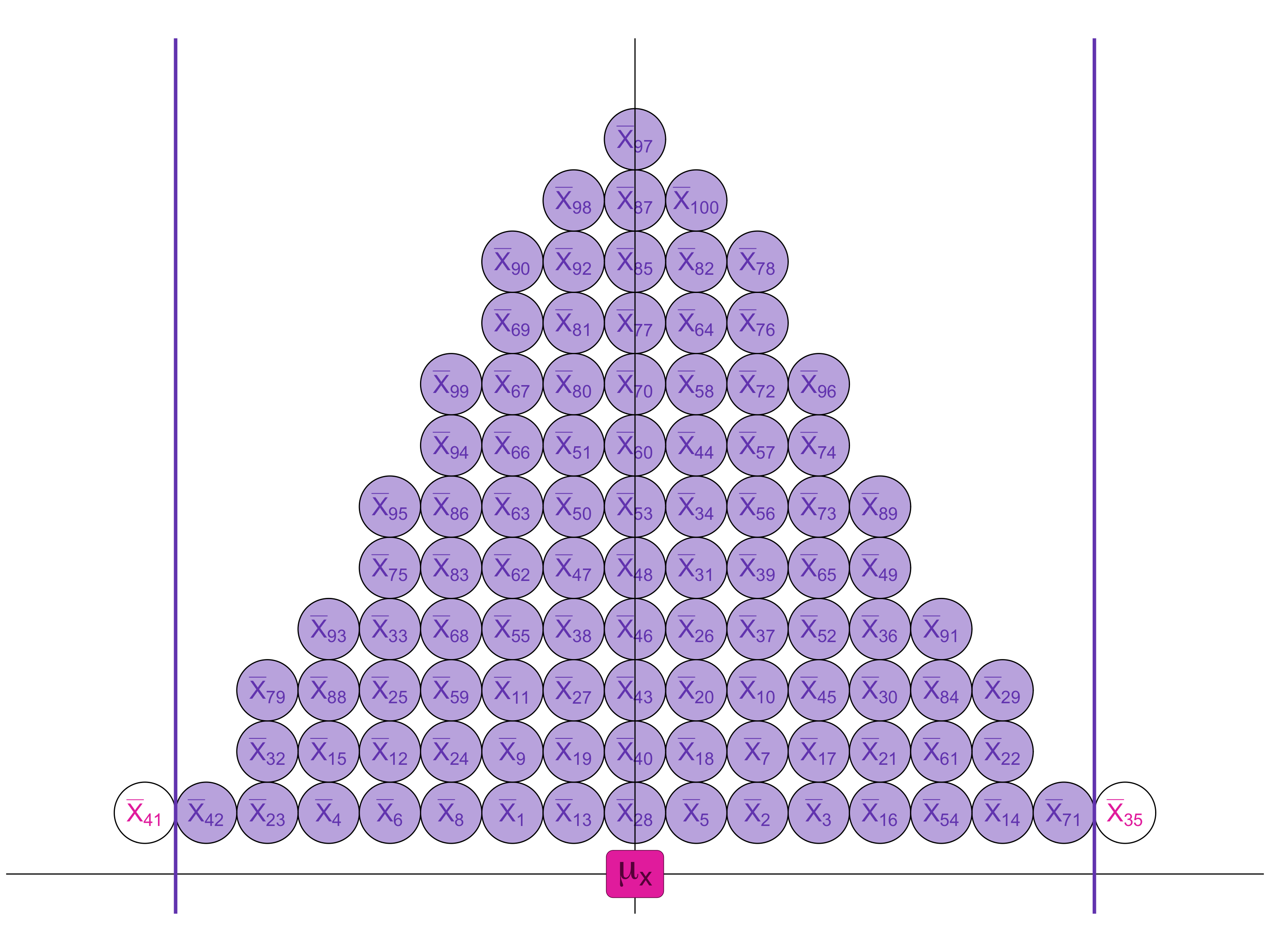
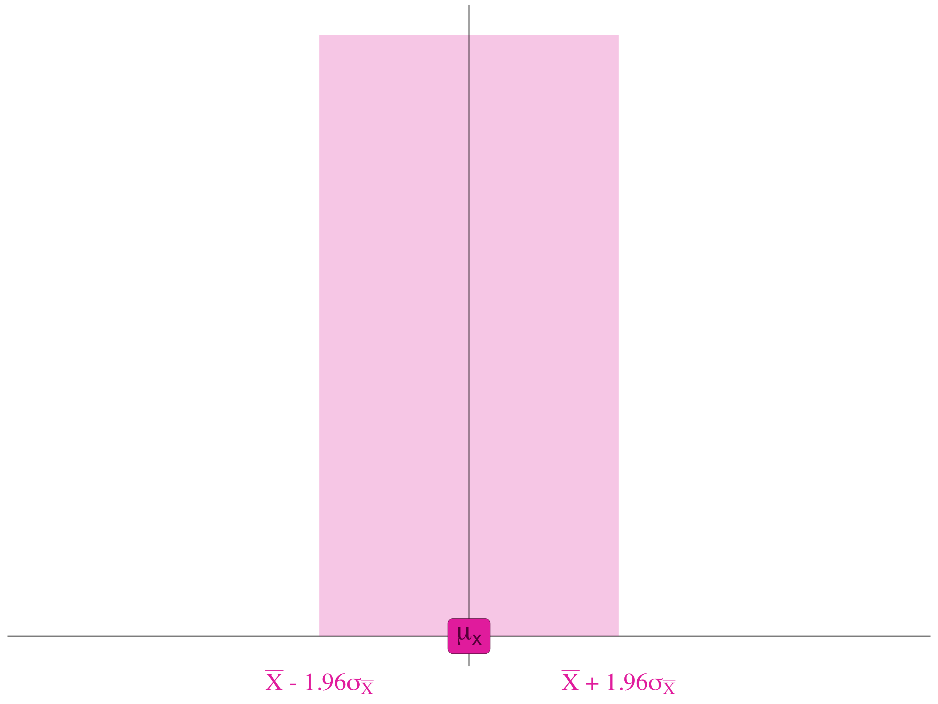
95% of sample means will be within 1.96 \(\sigma\) of the pop. mean

Sampling Distribution

Important facts about sampling distributions:

• Theoretical distributions: can’t take every possible sample from the population
• Each statistic that we might be interested in has a theoretical sampling distribution
• Just by chance, the different samples making up this sampling distribution will give different statistics
  • e.g., the mean for each sample will probably be slightly different because different individuals make up the different samples.
  • Reflects chance sampling error.
• “Probability distribution” means that if we know the shape of the distribution we can find the probability of a particular sample score within the distribution of all the possible sample scores

Three types of distributions

Break!

Central limit theorem

Central Limit Theorem (CLT)

If all possible random samples of size \(N\) are drawn from a population with the mean \(\mu_X\) and the standard deviation \(\sigma_X\), then as \(N\) becomes larger, the sampling distribution of the sample means becomes approximately normal, with mean equal to \(\mu_X\) and standard deviation equal to the population standard deviation divided by square root of the sample size.

Implication of central limit theorem

• Central limit theorem tells us that if the size of our random sample is large enough, we can assume that the sampling distribution of all such possible samples is:
  • Normally distributed
  • Mean: \(\mu_\bar{X}\) \(= \mu_X\)

Implication of central limit theorem

• Central limit theorem tells us that if the size of our random sample is large enough, we can assume that the sampling distribution of all such possible samples is:
  • Normally distributed
  • Mean: \(\mu_\bar{X}\) \(= \mu_X\)

Check out this new symbol:
The population mean of sample means
(i.e., the average of the means you would
calculate from all possible samples)

Implication of central limit theorem

• Central limit theorem tells us that if the size of our random sample is large enough, we can assume that the sampling distribution of all such possible samples is:
  • Normally distributed
  • Mean: \(\mu_\bar{X}\) \(= \mu_X\)
  • Standard Error = \(\sigma_\bar{X}\) \(= \frac{\sigma}{\sqrt{n}}\)

Standard error:
The standard deviation in
the sampling distribution
(in this case, of all
possible sample means)

Implication of central limit theorem

• Central limit theorem tells us that if the size of our random sample is large enough, we can assume that the sampling distribution of all such possible samples is:
  • Normally distributed
  • Mean: \(\mu_\bar{X}\) \(= \mu_X\)
  • Standard Error = \(\sigma_\bar{X}\) \(= \frac{\sigma}{\sqrt{n}}\)

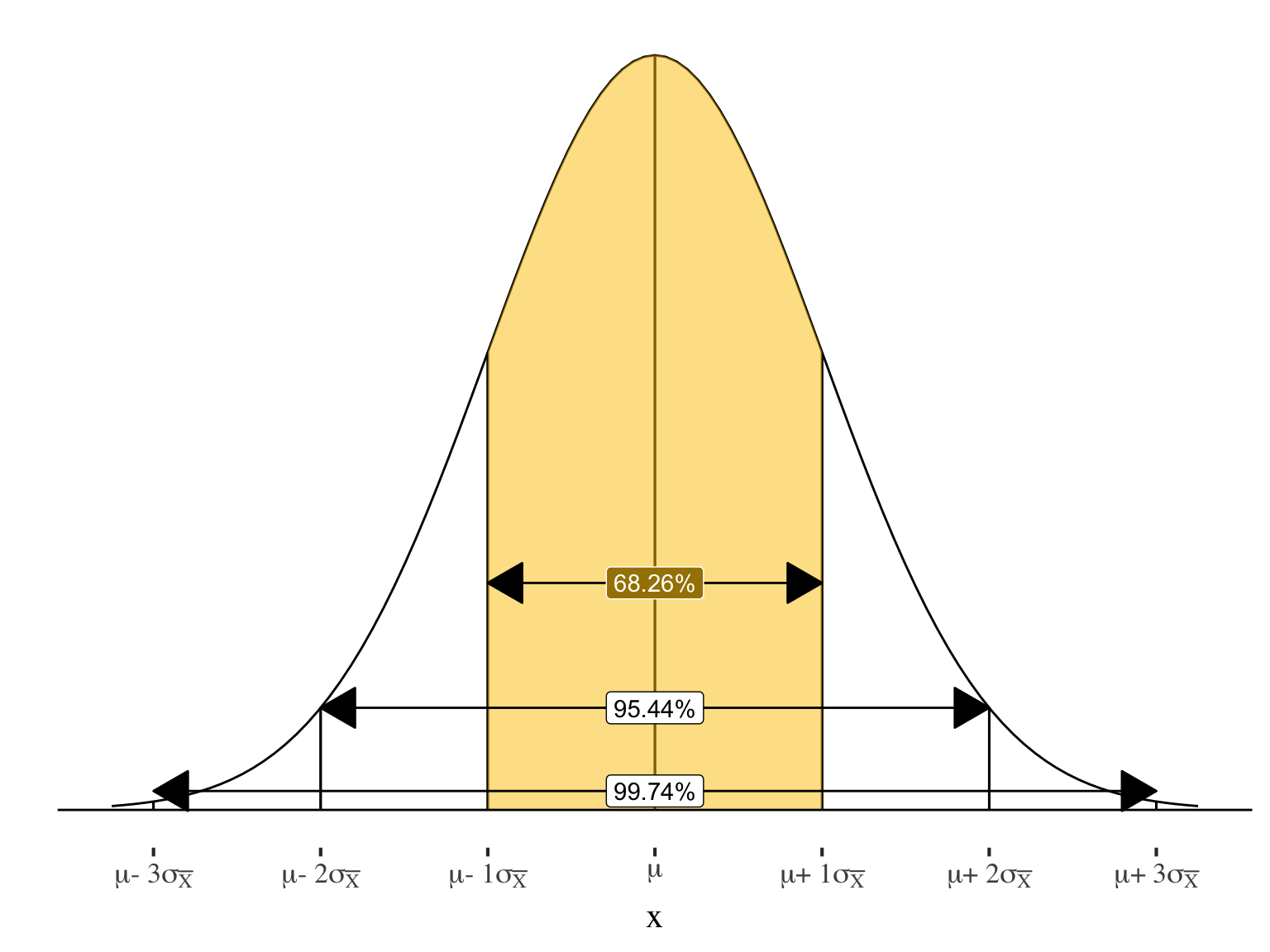
Just over 68% of sample means will be within ±1 standard error of the true population mean

Implication of central limit theorem

• Central limit theorem tells us that if the size of our random sample is large enough, we can assume that the sampling distribution of all such possible samples is:
  • Normally distributed
  • Mean: \(\mu_\bar{X}\) \(= \mu_X\)
  • Standard Error = \(\sigma_\bar{X}\) \(= \frac{\sigma}{\sqrt{n}}\)

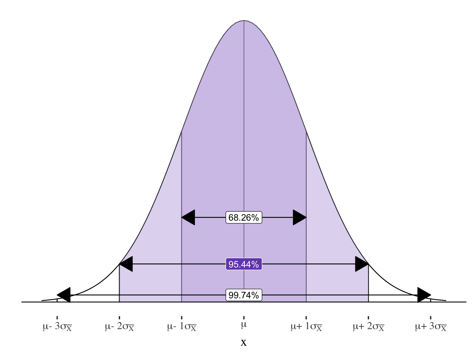
\(95.44\%\) of sample means will be within \(\pm2\) standard errors of the true population mean

And exactly \(95\%\) will be within \(1.96\) standard errors

Implication of central limit theorem

• Central limit theorem tells us that if the size of our random sample is large enough, we can assume that the sampling distribution of all such possible samples is:
  • Normally distributed
  • Mean: \(\mu_\bar{X}\) \(= \mu_X\)
  • Standard Error = \(\sigma_\bar{X}\) \(= \frac{\sigma}{\sqrt{n}}\)

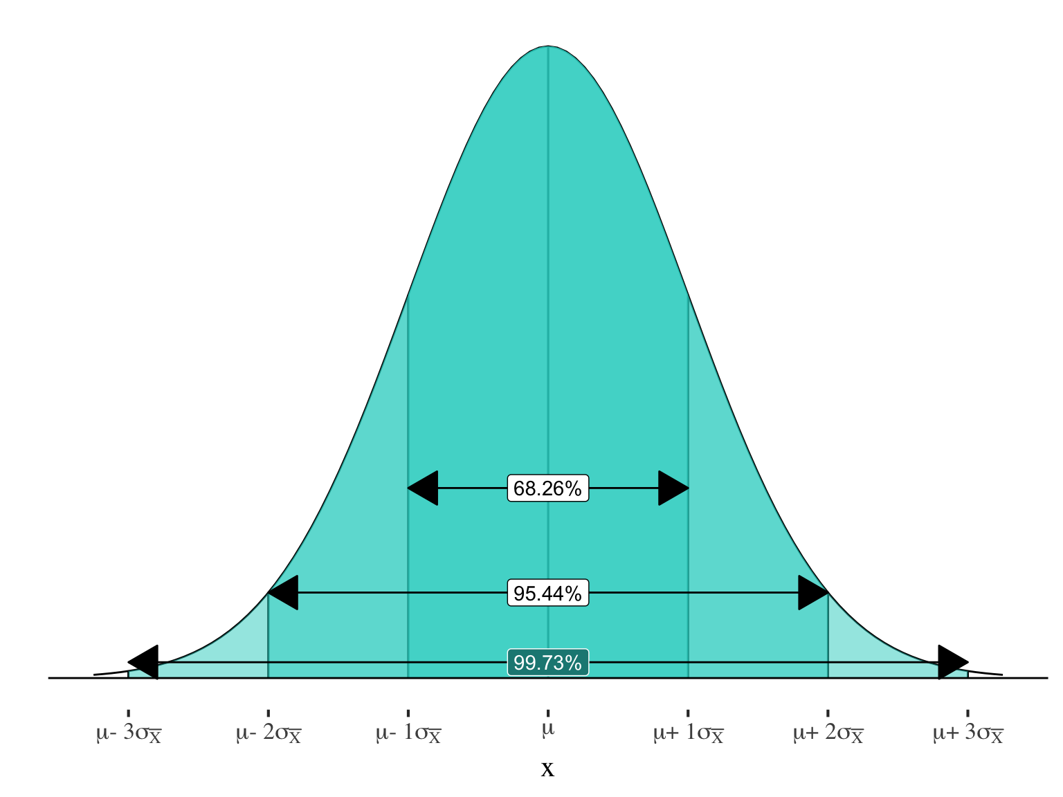
\(99.73\%\) of sample means will be within \(\pm3\) standard errors of the true population mean

How does this help us?

SAMPLING DISTRIBUTION of sample means

If, 95% of the samples are within 1.96 standard errors of the true population mean . . .

If, 95% of the samples are within 1.96 standard errors of the true population mean . . .

. . . then for 95 samples out of 100, we will find the true population mean if we look within 1.96 standard errors of the sample mean.

If, 95% of the samples are within 1.96 standard errors of the true population mean . . .

. . . then for 95 samples out of 100, we will find the true population mean if we look within 1.96 standard errors of the sample mean.

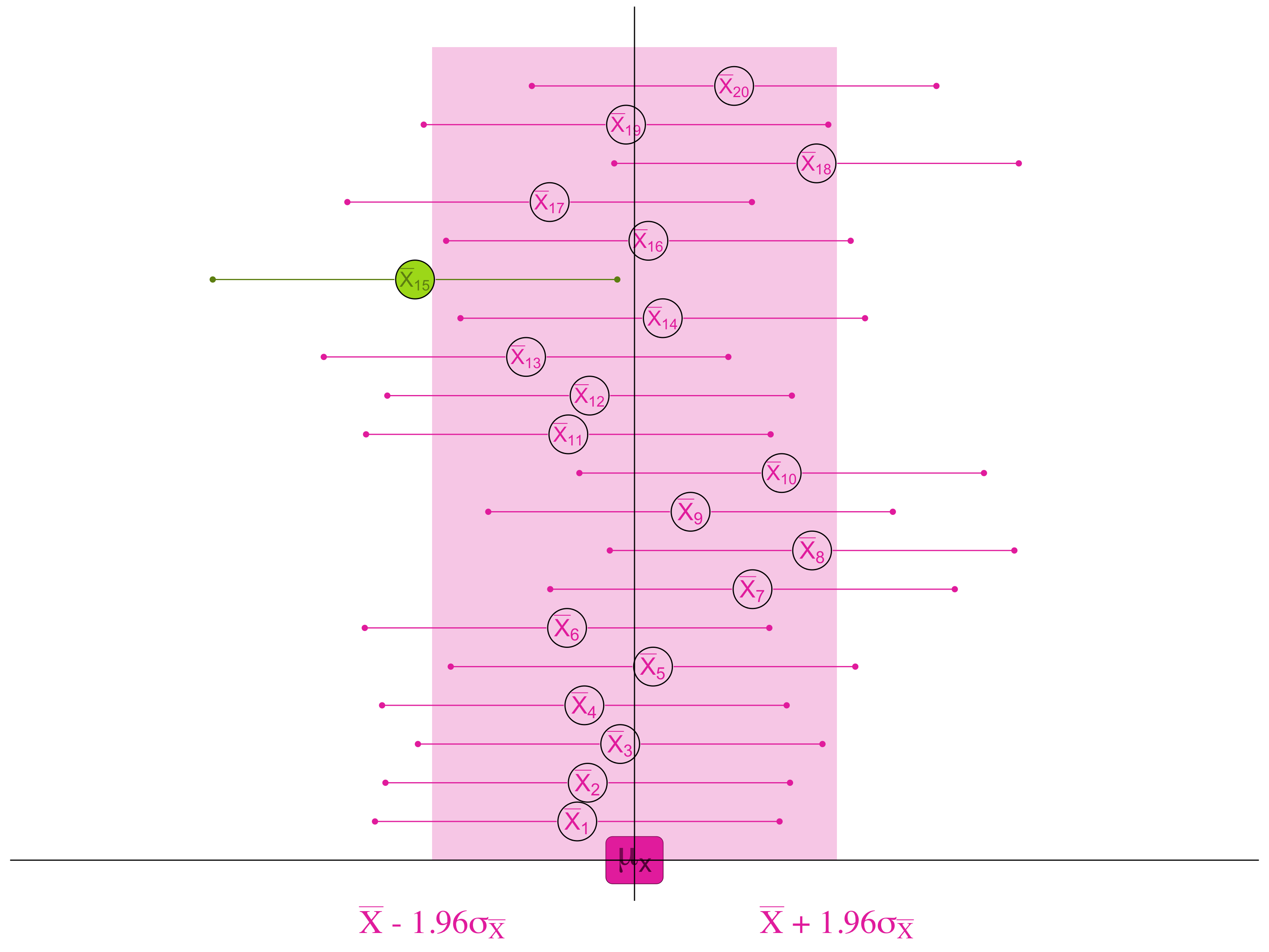
If, 95% of the samples are within 1.96 standard errors of the true population mean . . .

. . . then for 95 samples out of 100, we will find the true population mean if we look within 1.96 standard errors of the sample mean.

Confidence intervals

The BIG IDEA:

• The sampling distribution and CLT tells us how close to the population mean (\(\mu\)) the sample mean (\(\bar{X}\)) is likely to be
• We can use this knowledge to figure out how close the true population mean (\(\mu\)) is likely to be to the one sample mean (\(\bar{X}\))that we observe
• Build a confidence interval around our sample statistic (mean) to define the range in which we think the population parameter can be found…
  • … and quantify how likely it is that we are right

Using these tools for inference

Example: Want to know how much UW students study on average

\(\bar{X}\) —INFERENCE–> \(\mu_x\)

Sample statistic: The characteristic of the sample that we actually observe (i.e. the mean study time of a SAMPLE of UW students)

For example: draw a random sample of 100 students and observe \(\bar{X} = 14.5\)

Population parameter: The characteristic of the population that we are interested in knowing (i.e. the mean study time of all UW students)

Our goal: Estimate the unknown population parameter \(\mu_x = ?\)

Confidence intervals

\[ \bar{X} \]

Create a range of scores, centered on the sample mean, in which we think the population mean is likely to be located

Building a margin of error around our sample mean

Confidence interval:
\(\text{sample statistic} \pm \text{margin of error}\)

⬅️

All confidence intervals take this form

Practice

Problem 1: Sampling Distributions

A researcher is studying weekly TV viewing habits of college students. The population mean is unknown, but the population standard deviation is \(\sigma = 5\) hours.

Suppose a simple random sample of \(n = 100\) students is taken, and the sample mean viewing time is \(\bar{X}\) = 12 hours.

1. What is the standard error of the sample mean?
2. According to the Central Limit Theorem, what is the shape of the sampling distribution of \(\bar{X}\)? Why?
3. Would the standard error be larger, smaller, or the same if the sample size were only 25? Explain your reasoning.

Problem 1: Sampling Distributions

1. Standard Error:
   \[ SE = \frac{\sigma}{\sqrt{n}} = \frac{5}{\sqrt{100}} = 0.5 \text{ hours} \]
   

2. Shape of Sampling Distribution:
   Since \(n = 100\) is large, by the Central Limit Theorem, the sampling distribution of \(\bar{X}\) is approximately normal, regardless of population shape.
   

3. What if \(n = 25\)?
   \[ SE = \frac{5}{\sqrt{25}} = 1.0 \]
   So the standard error increases when sample size decreases.

Practice

Problem 2: Central Limit Theorem

Imagine a population where the distribution of individual income is strongly skewed right with a mean of $50,000 and a standard deviation of $10,000.

1. If we take a random sample of 5 people, will the distribution of the sample mean look approximately normal? Why or why not?
2. What about a sample of 50 people?
3. Explain why the CLT is important for making inferences using sample means, even when the population distribution is not normal.

Problem 2: Central Limit Theorem

1. \(n = 5\): The sampling distribution of \(\bar{X}\) is not approximately normal — small sample from a strongly skewed population.
   

2. \(n = 50\): Sampling distribution is approximately normal — CLT applies for large enough \(n\) (typically \(n \geq 30\)).
   

3. Why is CLT useful?
   It allows us to use the normal model for sample means even when the population is not normal, as long as \(n\) is large.

Practice

Problem 3: Comparing Sample Means

Two different researchers each take a simple random sample from the same population of high school students.

• Researcher A: \(n = 30\), gets \(\bar{X}_A = 7\) hours of sleep per night
• Researcher B: n = 90, gets \(\bar{X}_B = 7.2\) hours of sleep per night
• The population standard deviation is known to be \(\sigma\) = 1.8 hours

1. Who would have a smaller standard error, and why?
2. Without calculating exact probabilities, which researcher is more likely to have a sample mean close to the true population mean?
3. What does this example illustrate about the relationship between sample size and variability in sample statistics?

Problem 3: Comparing Sample Means

1. Standard Errors: \[ SE_A = \frac{1.8}{\sqrt{30}} \approx 0.33 \qquad SE_B = \frac{1.8}{\sqrt{90}} \approx 0.19 \]
   So Researcher B has a smaller standard error.
   

2. Who is closer to \(\mu\)?
   Researcher B — lower SE means their estimate is more precise.
   

3. What does this show?
   Larger sample sizes → smaller SE → less variability in sample means.