Probability and probability distributions
& Normal distributions
SOC 221 • Lecture 4
Monday, July 1, 2024
Myths about randomness and probability
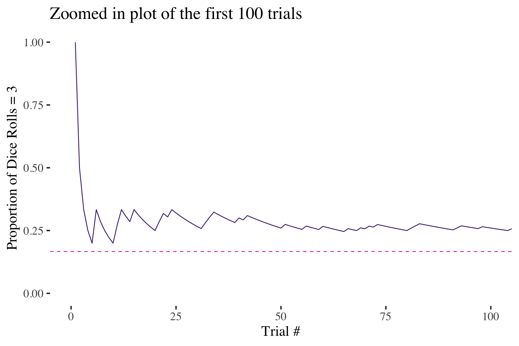
The myth of short-run regularity
Myth: If I flip a coin 10 times I should get 5 heads.
Reality: Over a short number of flips, you might get lots of heads or lots of tails. Probabilities express expectations only over the long run.
There is a difference between theoretical probability (long run) and short-run experimental probability
Probability distribution
Probability distribution
For a random variable,
this specifies its
possible values
and their probabilities.
A discrete random variable X has separate values (such as 1,2, 3…) as its possible outcomes
Its probability distribution assigns a probability P(x) to each possible value of X
The sum of the probabilities for all the possible x values equals 1
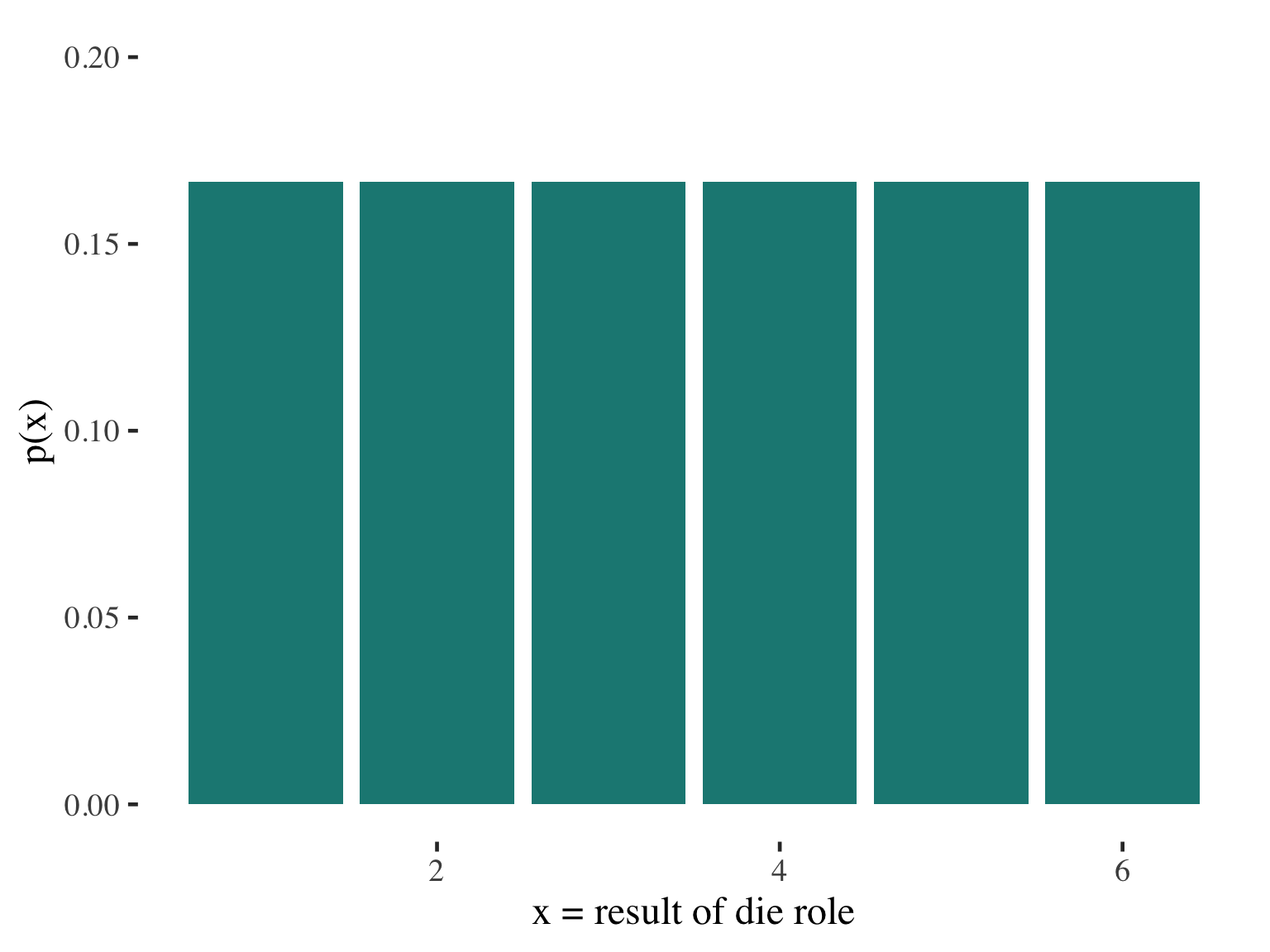
For each x, the probability P(x) falls between 0 and 1
Example: Probability distribution
What is the probability of a correct guess (choosing randomly) on a five-choice test question?
Probability distribution of guess outcomes
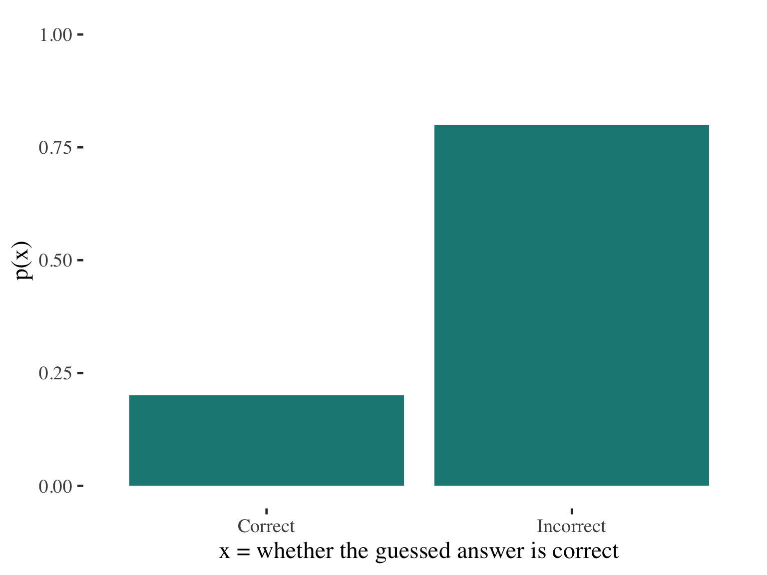
\[ P(C) = \frac{1}{5} = 0.2 \]
\[ P(I) = \frac{4}{5} = 0.8 \]
Note (again!):
Probabilities = Proportions
Example: Probability distribution
Probability distributions are reflected in frequency distributions
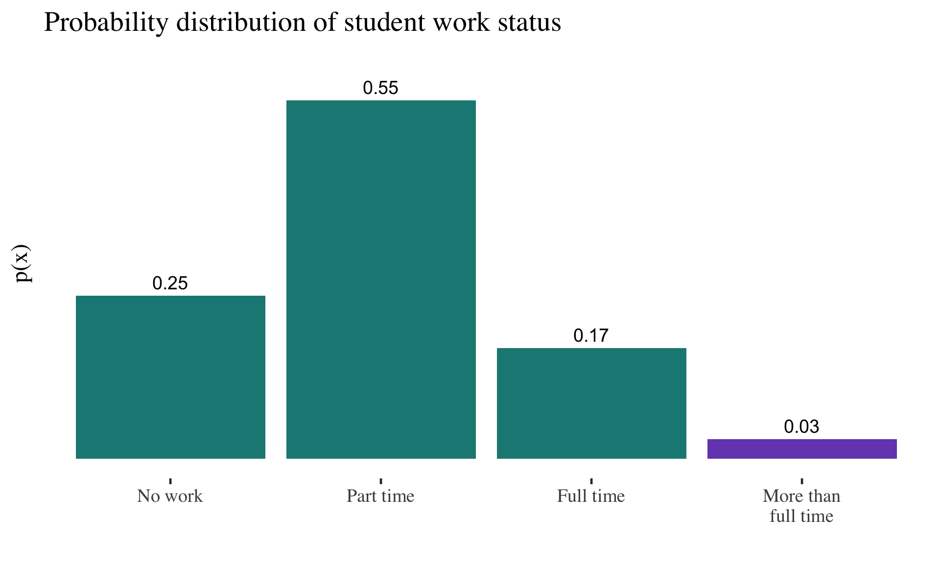
As long as every possible outcome is included, we can think of this as a probability distribution
For example: The
probability of randomly selecting a student who works more than full time is .03
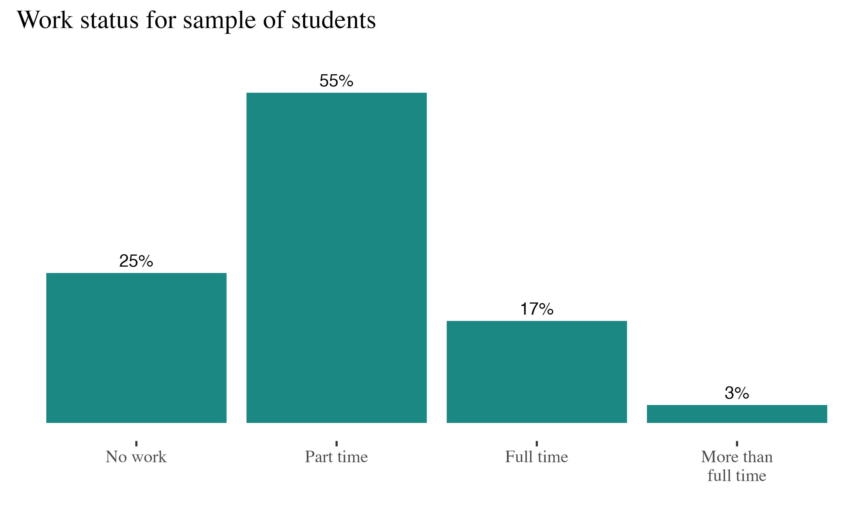
Examples: What is the probability of randomly selecting…
A single student who does not work?
Two consecutive students who do not work?
A single student who works at least full time?
Examples: What is the probability of randomly selecting…
A single student who does not work?
\(P(nw) = 0.25\)
Examples: What is the probability of randomly selecting…
Two consecutive students who do not work?
\(P(\text{nw, nw}) = (0.25)(0.25) = 0.0625\)
Examples: What is the probability of randomly selecting…
A single student who works at least full time?
\(P(\text{ft or mft}) = 0.17 + 0.03 = 0.20\)
Examples: Probability distribution
Probability distributions are reflected in frequency distribution
Discrete probability distribution
Shows the probability of
a set of distinct,
separable outcomes.
Examples: Continuous probability distribution
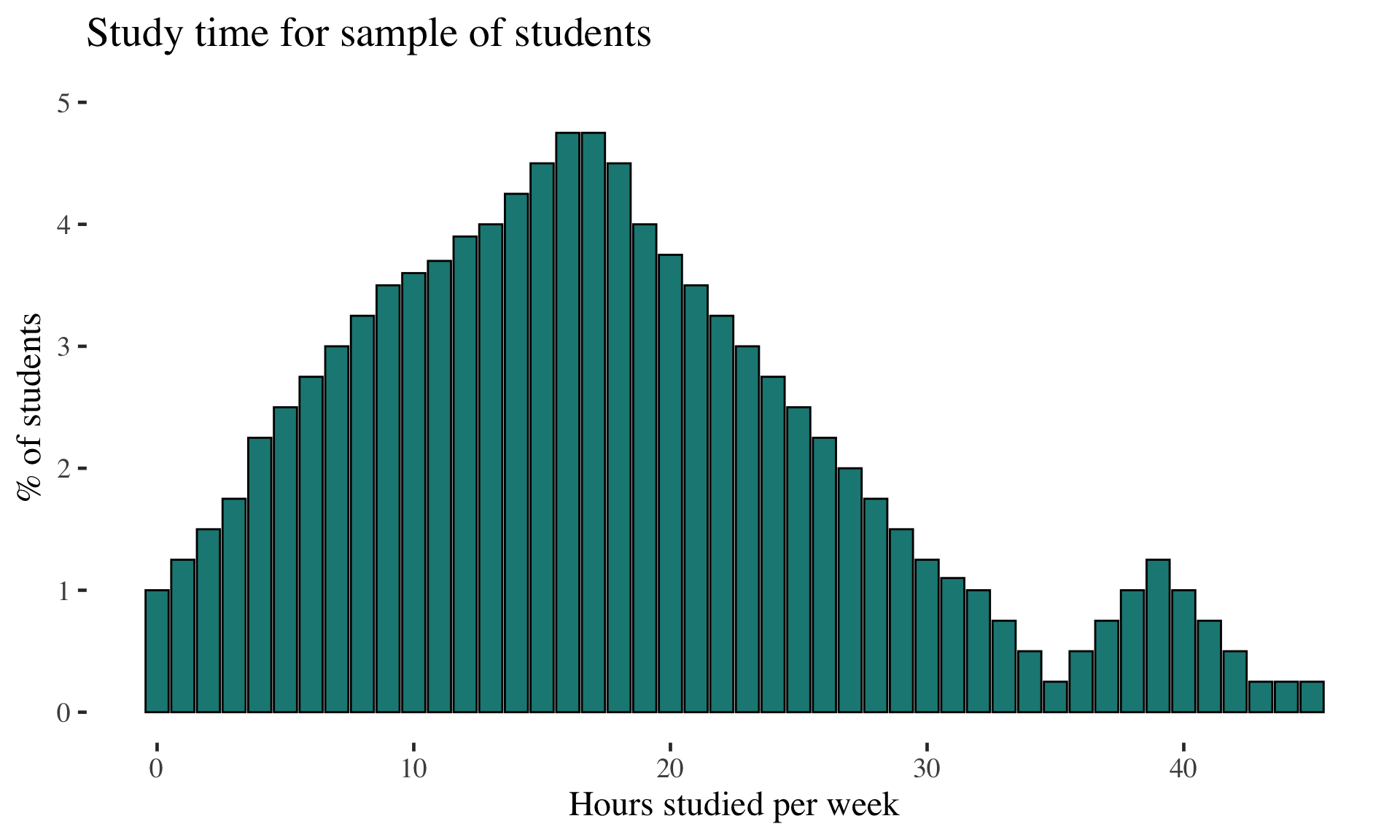
Probability density function
Shows the probability of a
set of continuous outcomes.
Can use a histogram to create a continuous probability distribution
Note: Continuous random variables have an infinite continuum of possible values in an interval (e.g., time, age, height, weight…)
Contrast to a discrete random variable (limited number of possible values)
Examples: Continuous probability distribution
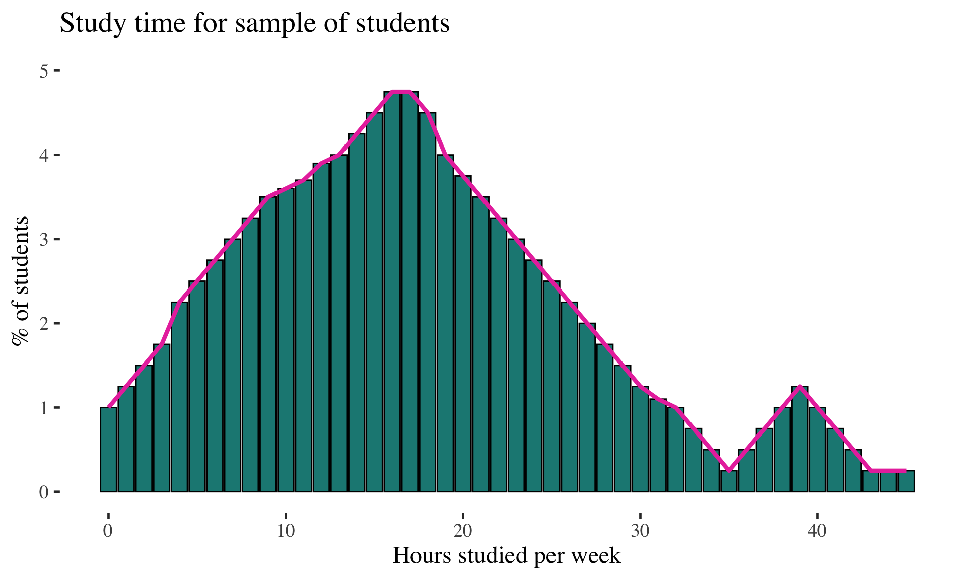
Just smooth out the distribution
Can describe probabilities of observing values within a range under the curve
Examples: Continuous probability distribution
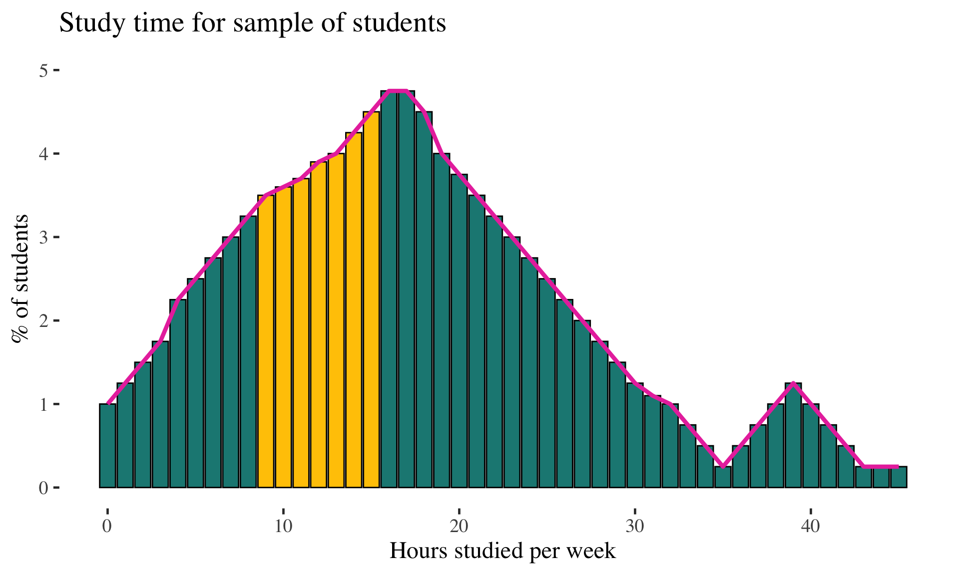
Just smooth out the distribution
Can describe probabilities of observing values within a range under the curve
EXAMPLE: If we know that 28.39% of students study between 9 and 15 hours, the probability of selecting a student from this range is .2839
Takeaway: Probability Distribution of a Continuous Random Variable
- A continuous random variable has possible values that form a curve (smoothing a histogram)
- Sometimes called a probability density function (pdf)
- Can think about probability of outcomes within a specific interval (range or a section under the curve)
- Probability = area under the curve for that interval
- Each interval has probability between 0 and 1
- The interval containing all possible values has probability equal to 1

How does this help us?

Characteristics of the
Normal Distribution
- Bell shaped
- Symmetric around the mean (and median and single mode)
- Declining frequencies on tails
- Both tails continue infinitely ever closer to 0 but without touching the baseline
←
NORMAL DISTRIBUTION
Continuous probability distribution
frequently used in inferentialstatistics
• Theoretical model
• But useful because:
1) its shape is well known
(familiar pdf); and
2) under certain conditions,
distributions that we need to
know about follow a normal
curve
Normal distribution
The mean (\(\mu\)) and the standard deviation (\(\sigma\)) completely describe the density curve for a normal distribution
- Increasing/decreasing \(\mu\) moves the curve along the horizontal axis
- Increasing/decreasing \(\sigma\) determines the spread of the curve
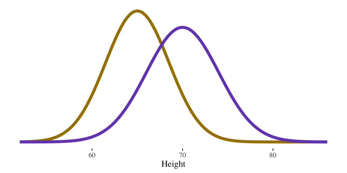
Women \(N(65, 3.5)\)
Men \(N(70, 4.0)\)
Consistent areas under the normal curve
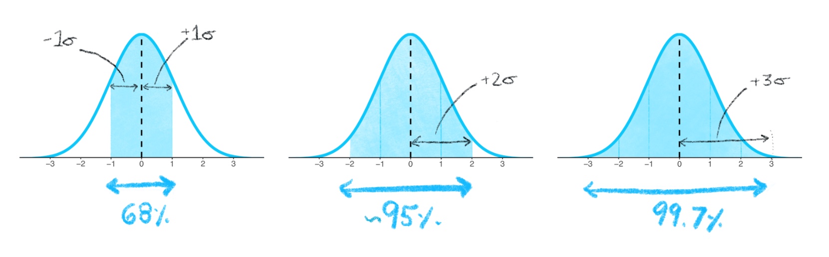
Empirical (68-95-99) Rule
For ANY Normal Curve
- 68.26% of the observations fall within one \(\sigma\) of the mean (\(\mu\))
- 95.44% of the observations fall within two \(\sigma\) of the mean (\(\mu\))
- 99.73% of the observations fall within three \(\sigma\) of the mean (\(\mu\))
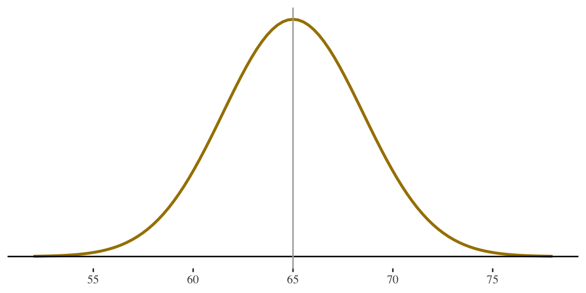
Example of consistent areas under the normal curve
- Heights of adult women
- Roughly follow a normal distribution
- \(\mu\) = 65 inches; \(\sigma\) = 3.5 inches
Also, probability of randomly selecting a woman who is between 54.5 and 75.5 inches is 99.73/100 = .9973
- Apply 68-95-99.7 Rule for women’s heights
- 68.26% are between 61.5 and 68.5 in.
- [ \(\mu \pm \sigma\) = 65 ± 3.5 ]
- 95.44% are between 58 and 72 inches
- [ \(\mu \pm \sigma\) = 65 ± 2(3.5) = 65 ± 7 ]
- 99.73% are between 54.5 and 75.5 inches
- [ \(\mu \pm \sigma\) = 65 ± 3(3.5) = 65 ± 10.5 ]
- 68.26% are between 61.5 and 68.5 in.
Women \(N(65, 3.5)\)
Example of consistent areas under the normal curve
Notice that when we are finding areas under the normal curve, we are always thinking in terms of standard deviation units
e.g., how many standard deviations away from the mean of the distribution are we?
Called a standard normal distribution
STEP 1
Draw the picture (highly recommended)
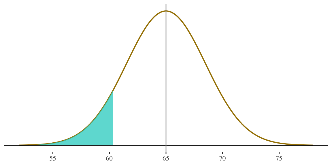
If height for women is \(N(65,3.5)\) what percentage of women are shorter than 5 feet tall (i.e., 60 inches)?
STEP 1
Draw the picture (highly recommended)
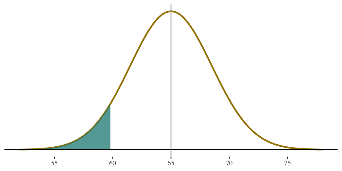
If height for women is \(N(65,3.5)\) what percentage of women are shorter than 5 feet tall (i.e., 60 inches)?
5 feet is 60 inches. I know that is somewhere below the mean, and I’m interested in the area below that point.
STEP 2
Convert value(s) of interest into z-score(s)

If height for women is \(N(65,3.5)\) what percentage of women are shorter than 5 feet tall (i.e., 60 inches)?
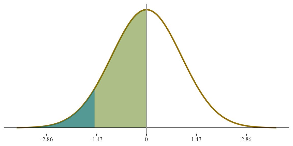
\[ z = \frac{60 - 65}{3.5} = -1.43 \]
5 feet is 1.43 standard deviations below average.
STEP 2
Convert value(s) of interest into z-score(s)

If height for women is \(N(65,3.5)\) what percentage of women are shorter than 5 feet tall (i.e., 60 inches)?
\[ z = \frac{60 - 65}{3.5} = -1.43 \]
5 feet is 1.43 standard deviations below average.
STEP 3
Use standard normal table\(^1\) to find proportion of cases between the mean and the z-score

If height for women is \(N(65,3.5)\) what percentage of women are shorter than 5 feet tall (i.e., 60 inches)?
Table will give us this area
\(^1\)A standard normal table can be found here
How to use a standard normal (z-score) table
| 0 | 0.1 | 0.2 | 0.3 | 0.4 | 0.5 | 0.6 | 0.7 | 0.8 | 0.9 | 1 | 1.1 | 1.2 | 1.3 | 1.4 | 1.5 | 1.6 | 1.7 | 1.8 | 1.9 | 2 | 2.1 | 2.2 | 2.3 | 2.4 | 2.5 | 2.6 | 2.7 | 2.8 | 2.9 | 3 | 3.1 | 3.2 | 3.3 | 3.4 | |
|---|---|---|---|---|---|---|---|---|---|---|---|---|---|---|---|---|---|---|---|---|---|---|---|---|---|---|---|---|---|---|---|---|---|---|---|
| 0 | 0.000000 | 0.03983 | 0.07926 | 0.1179 | 0.1554 | 0.1915 | 0.2257 | 0.2580 | 0.2881 | 0.3159 | 0.3413 | 0.3643 | 0.3849 | 0.4032 | 0.4192 | 0.4332 | 0.4452 | 0.4554 | 0.4641 | 0.4713 | 0.4772 | 0.4821 | 0.4861 | 0.4893 | 0.4918 | 0.4938 | 0.4953 | 0.4965 | 0.4974 | 0.4981 | 0.4987 | 0.4990 | 0.4993 | 0.4995 | 0.4997 |
| 0.01 | 0.003989 | 0.04380 | 0.08317 | 0.1217 | 0.1591 | 0.1950 | 0.2291 | 0.2611 | 0.2910 | 0.3186 | 0.3438 | 0.3665 | 0.3869 | 0.4049 | 0.4207 | 0.4345 | 0.4463 | 0.4564 | 0.4649 | 0.4719 | 0.4778 | 0.4826 | 0.4864 | 0.4896 | 0.4920 | 0.4940 | 0.4955 | 0.4966 | 0.4975 | 0.4982 | 0.4987 | 0.4991 | 0.4993 | 0.4995 | 0.4997 |
| 0.02 | 0.007978 | 0.04776 | 0.08706 | 0.1255 | 0.1628 | 0.1985 | 0.2324 | 0.2642 | 0.2939 | 0.3212 | 0.3461 | 0.3686 | 0.3888 | 0.4066 | 0.4222 | 0.4357 | 0.4474 | 0.4573 | 0.4656 | 0.4726 | 0.4783 | 0.4830 | 0.4868 | 0.4898 | 0.4922 | 0.4941 | 0.4956 | 0.4967 | 0.4976 | 0.4982 | 0.4987 | 0.4991 | 0.4994 | 0.4995 | 0.4997 |
| 0.03 | 0.011966 | 0.05172 | 0.09095 | 0.1293 | 0.1664 | 0.2019 | 0.2357 | 0.2673 | 0.2967 | 0.3238 | 0.3485 | 0.3708 | 0.3907 | 0.4082 | 0.4236 | 0.4370 | 0.4484 | 0.4582 | 0.4664 | 0.4732 | 0.4788 | 0.4834 | 0.4871 | 0.4901 | 0.4925 | 0.4943 | 0.4957 | 0.4968 | 0.4977 | 0.4983 | 0.4988 | 0.4991 | 0.4994 | 0.4996 | 0.4997 |
| 0.04 | 0.015953 | 0.05567 | 0.09483 | 0.1331 | 0.1700 | 0.2054 | 0.2389 | 0.2704 | 0.2995 | 0.3264 | 0.3508 | 0.3729 | 0.3925 | 0.4099 | 0.4251 | 0.4382 | 0.4495 | 0.4591 | 0.4671 | 0.4738 | 0.4793 | 0.4838 | 0.4875 | 0.4904 | 0.4927 | 0.4945 | 0.4959 | 0.4969 | 0.4977 | 0.4984 | 0.4988 | 0.4992 | 0.4994 | 0.4996 | 0.4997 |
| 0.05 | 0.019939 | 0.05962 | 0.09871 | 0.1368 | 0.1736 | 0.2088 | 0.2422 | 0.2734 | 0.3023 | 0.3289 | 0.3531 | 0.3749 | 0.3944 | 0.4115 | 0.4265 | 0.4394 | 0.4505 | 0.4599 | 0.4678 | 0.4744 | 0.4798 | 0.4842 | 0.4878 | 0.4906 | 0.4929 | 0.4946 | 0.4960 | 0.4970 | 0.4978 | 0.4984 | 0.4989 | 0.4992 | 0.4994 | 0.4996 | 0.4997 |
| 0.06 | 0.023922 | 0.06356 | 0.10257 | 0.1406 | 0.1772 | 0.2123 | 0.2454 | 0.2764 | 0.3051 | 0.3315 | 0.3554 | 0.3770 | 0.3962 | 0.4131 | 0.4279 | 0.4406 | 0.4515 | 0.4608 | 0.4686 | 0.4750 | 0.4803 | 0.4846 | 0.4881 | 0.4909 | 0.4931 | 0.4948 | 0.4961 | 0.4971 | 0.4979 | 0.4985 | 0.4989 | 0.4992 | 0.4994 | 0.4996 | 0.4997 |
| 0.07 | 0.027903 | 0.06749 | 0.10642 | 0.1443 | 0.1808 | 0.2157 | 0.2486 | 0.2794 | 0.3078 | 0.3340 | 0.3577 | 0.3790 | 0.3980 | 0.4147 | 0.4292 | 0.4418 | 0.4525 | 0.4616 | 0.4693 | 0.4756 | 0.4808 | 0.4850 | 0.4884 | 0.4911 | 0.4932 | 0.4949 | 0.4962 | 0.4972 | 0.4979 | 0.4985 | 0.4989 | 0.4992 | 0.4995 | 0.4996 | 0.4997 |
| 0.08 | 0.031881 | 0.07142 | 0.11026 | 0.1480 | 0.1844 | 0.2190 | 0.2517 | 0.2823 | 0.3106 | 0.3365 | 0.3599 | 0.3810 | 0.3997 | 0.4162 | 0.4306 | 0.4429 | 0.4535 | 0.4625 | 0.4699 | 0.4761 | 0.4812 | 0.4854 | 0.4887 | 0.4913 | 0.4934 | 0.4951 | 0.4963 | 0.4973 | 0.4980 | 0.4986 | 0.4990 | 0.4993 | 0.4995 | 0.4996 | 0.4997 |
| 0.09 | 0.035856 | 0.07535 | 0.11409 | 0.1517 | 0.1879 | 0.2224 | 0.2549 | 0.2852 | 0.3133 | 0.3389 | 0.3621 | 0.3830 | 0.4015 | 0.4177 | 0.4319 | 0.4441 | 0.4545 | 0.4633 | 0.4706 | 0.4767 | 0.4817 | 0.4857 | 0.4890 | 0.4916 | 0.4936 | 0.4952 | 0.4964 | 0.4974 | 0.4981 | 0.4986 | 0.4990 | 0.4993 | 0.4995 | 0.4997 | 0.4998 |
- Number in the body of the table gives us the PROPORTION of cases between the mean and our positive z-value. Since the z-distribution is symmetrical, this is the same as the proportion between the mean and the corresponding negative z-value.
STEP 3
Use standard normal table\(^1\) to find proportion of cases between the mean and the z-score
If height for women is \(N(65,3.5)\) what percentage of women are shorter than 5 feet tall (i.e., 60 inches)?
Proportion in this area is .4236
\(^1\)A standard normal table can be found here
STEP 4
Subtract or add areas under the curve to get the total proportion you are looking for\(^1\)

If height for women is \(N(65,3.5)\) what percentage of women are shorter than 5 feet tall (i.e., 60 inches)?
Since we know that each half of
the distribution contains 50% of cases . . .
. . . and this area is .4236 . . .
\(^1\)see the picture from step 1
. . . the proportion in our shaded area is
0.50 - 0.4236 = 0.0764
STEP 5
Convert to percentages or probabilities as required by the problem

If height for women is \(N(65,3.5)\) what percentage of women are shorter than 5 feet tall (i.e., 60 inches)?
Multiply by 100 to get
from proportion to percentage:
\[
0.0764(100) = 7.636\%
\]
Answer: 7.64% of women
are shorter than 5 feet
. . . the proportion in our shaded area is
0.50 - 0.4236 = 0.0764
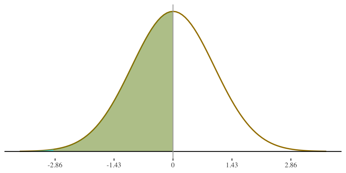
1. Percentage of women shorter than 55 inches?
Height for women is
\(N(65,3.5)\)
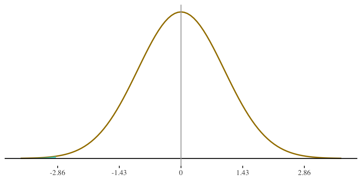
\[ z = \frac{55 - 65}{3.5} = -2.86 \]
55 inches is 2.86 standard deviations below the mean.
Now we look up the associated probability for our z-score
1. Percentage of women shorter than 55 inches?
Height for women is
\(N(65,3.5)\)
\[ z = \frac{55 - 65}{3.5} = -2.86 \]
This area is \(.49711\)
Proportion of cases under this shaded part of the curve is \(.50 - 0.49786 = 0.0021374\)
\[ \text{Percentage}(<55) = \] \[ 0.0021374(100) = \] \[ .214\% \]
2. Percentage of women 55 inches or taller?
Height for women is
\(N(65,3.5)\)
\[ z = \frac{55 - 65}{3.5} = -2.86 \]
55 inches is 2.86 standard deviations below the mean.
\[ \text{Percentage}(\ge55) = \] \[ 100- 0.214 = \] \[ 99.786\% \]
3. Probability of randomly selecting a woman who is 69 inches or taller?
Height for women is
\(N(65,3.5)\)
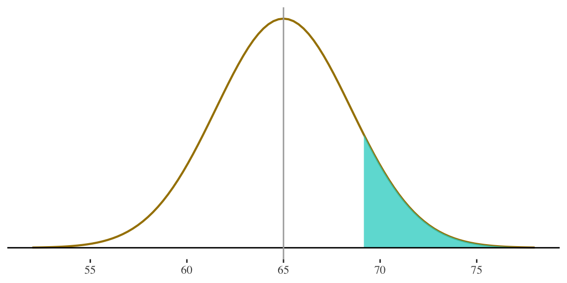
\[ z = \frac{69 - 65}{3.5} = 1.14 \]
69 inches is 1.14 standard deviations above the mean.
3. Probability of randomly selecting a woman who is 69 inches or taller?
Height for women is
\(N(65,3.5)\)
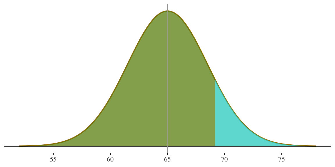
\[ z = \frac{69 - 65}{3.5} = 1.14 \]
69 inches is 1.14 standard deviations above the mean.
This area is \(0.50 + 0.37345 = 0.87345\) i.e. left half of the distribution plus the area between the mean and z-score of \(1.14\)
\[ P(\ge69) = \] \[ 1 - 0.87345 = \] \[ 0.12655 \]
4. Probability of randomly selecting two women, on consecutive draws, who are 69 inches or taller?
Height for women is
\(N(65,3.5)\)

\[ z = \frac{69 - 65}{3.5} = 1.14 \]
\[ P(\ge69) = \] \[ 1 - 0.87345 = \] \[ 0.12655 \]
Since BOTH events must happen, use the multiplication rule
\[ P(\ge69, \ge69) = \] \[ (0.12655)(0.12655) = \] \[ 0.016 \]
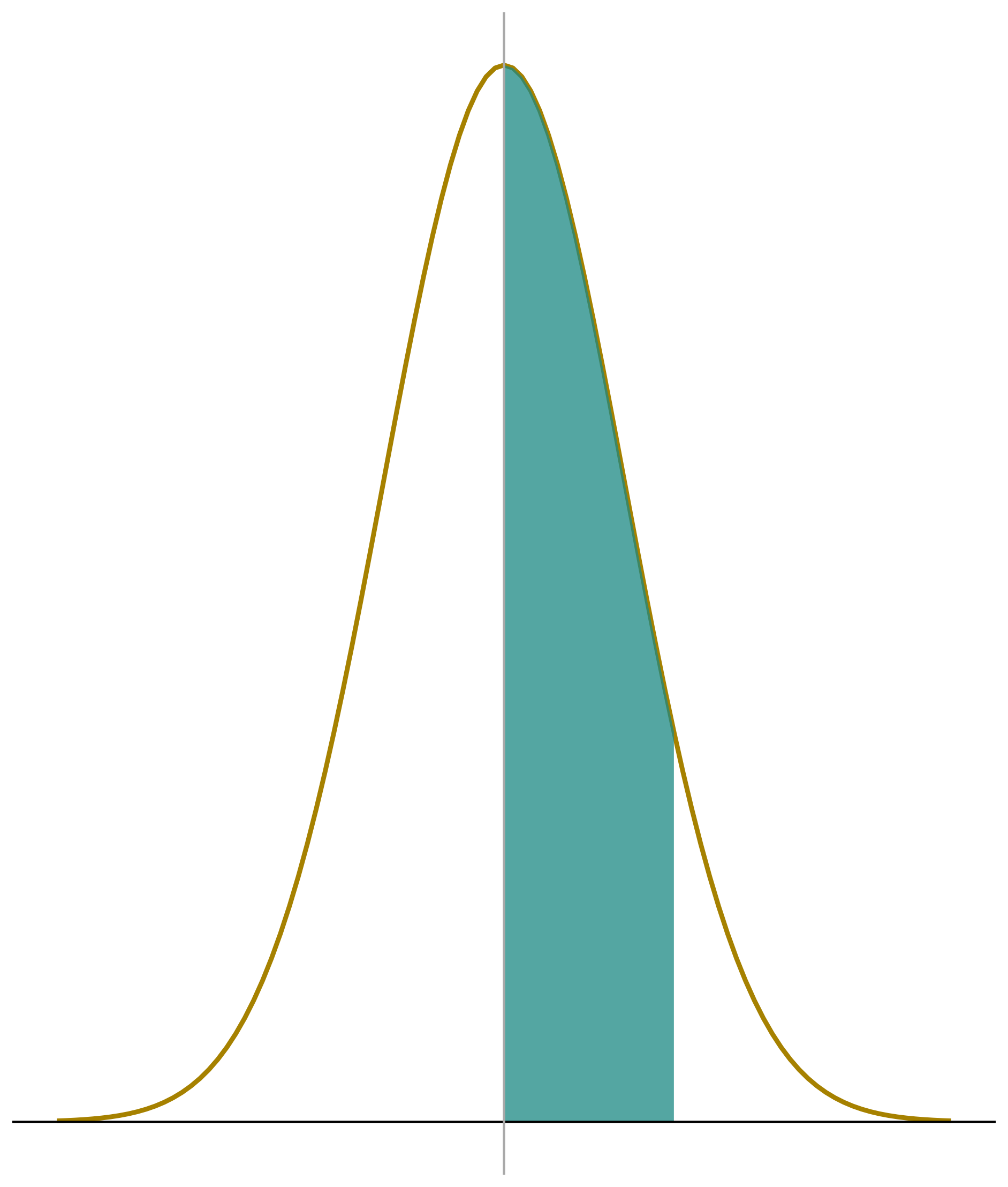
5. Find the score at the 10th percentile in the distribution.
Height for women is
\(N(65,3.5)\)
Now we look up the associated probability (\(0.10\)) to find our z-score
This shaded area represents the 10th percentile
5. Find the score at the 10th percentile in the distribution.
Height for women is
\(N(65,3.5)\)

The 10th percentile is associated with a z-score of \(-1.28\)
Instead of converting a value of
interest into a z-score . . . \[
z = \frac{X - \mu}{\sigma}
\]
. . . we need to convert our z-score
of interest into a value \[
X = \mu + z(\sigma)
\]
\[ X = 65 + (-1.28)(3.5) = 60.52 \]
Interpretation: The 10th percentile is at 60.52 inches. About 10% of women are 5 ft. ½ inch or shorter, and about 90% are taller.
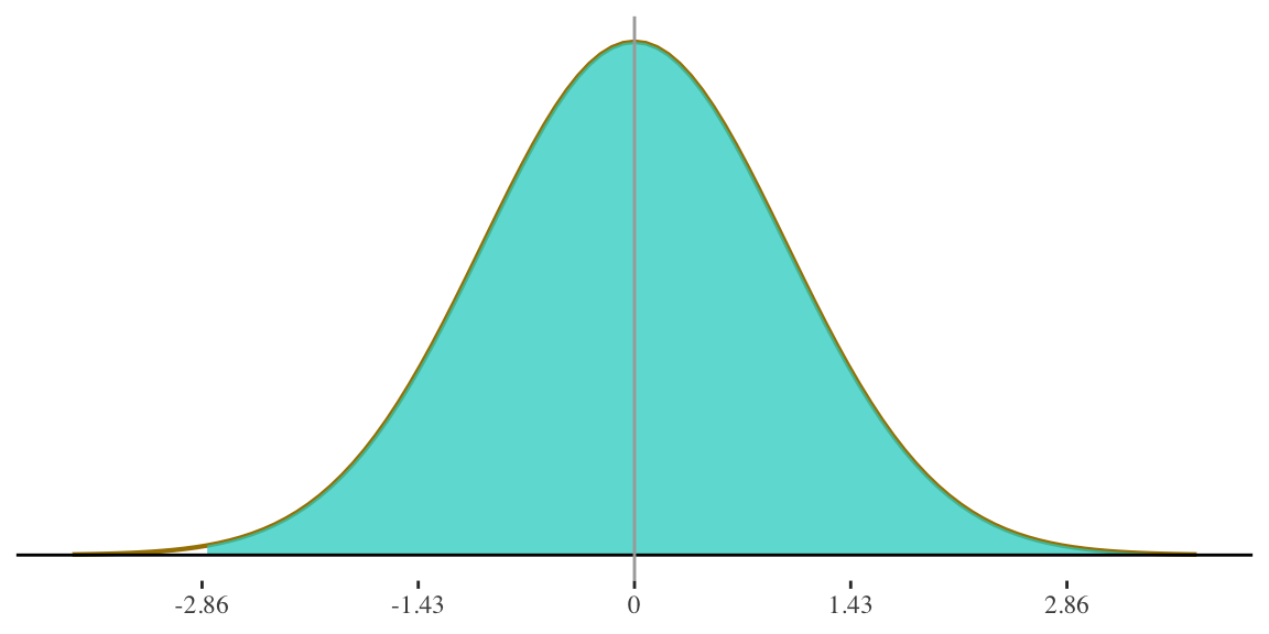
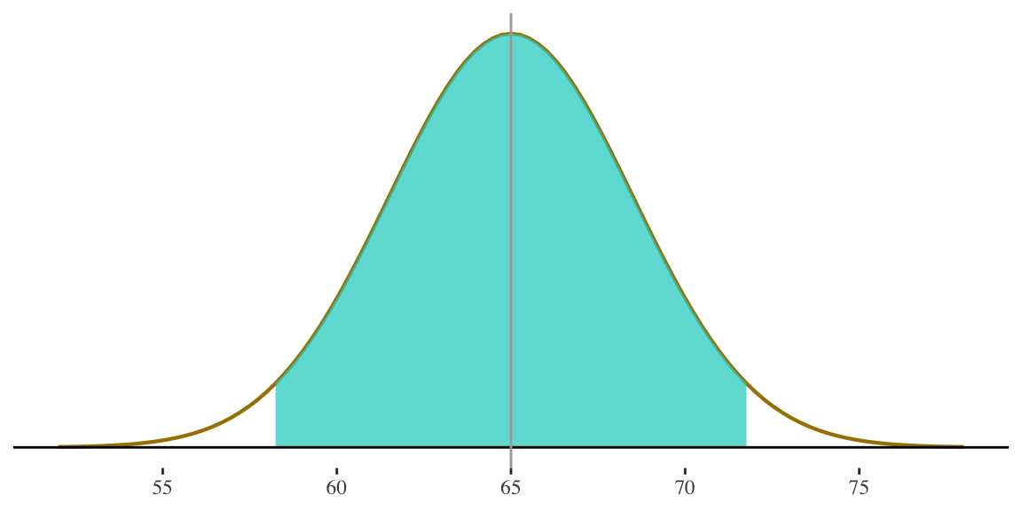
6. Find the two heights that define the middle 95% of cases in the distribution.
Height for women is
\(N(65,3.5)\)
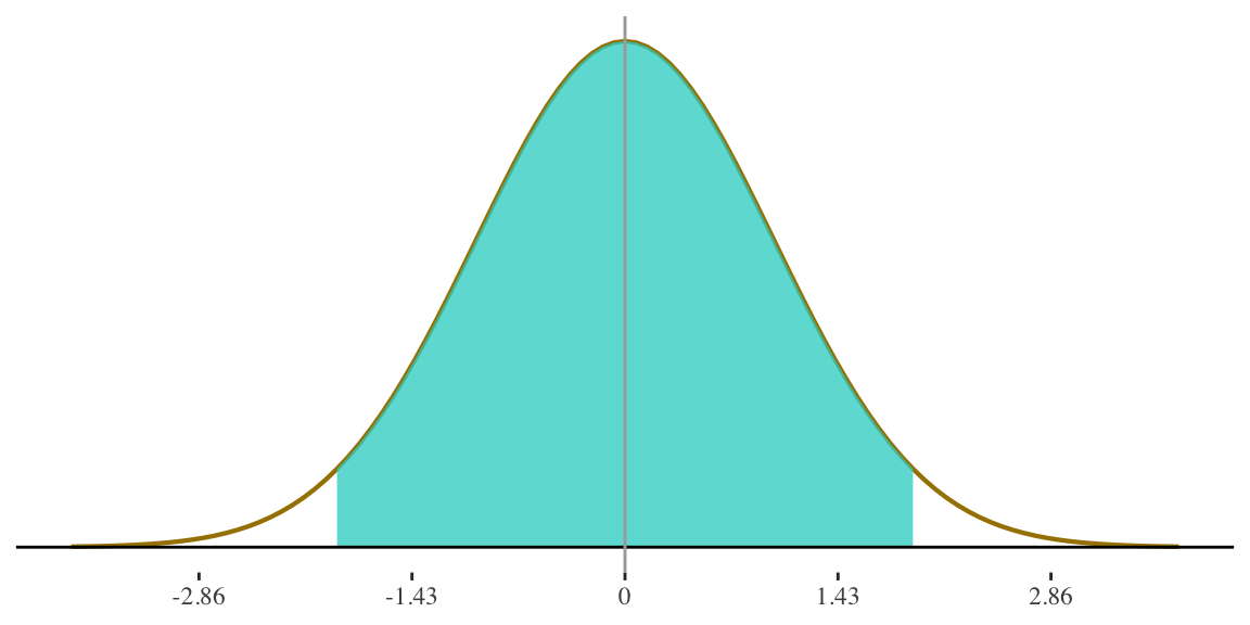
- Since capturing MIDDLE \(95\%\), we need to go the same direction above and below the mean
- How far on either side of the mean do we need to go in order to
capture \(\frac{95}{2} = 47.5\%\) of the cases?
Scores defining the middle 95% of cases (in any normal distribution) are at \(Z = -1.96\) and \(Z = 1.96\)
6. Find the two heights that define the middle 95% of cases in the distribution.
Height for women is
\(N(65,3.5)\)
- Since capturing MIDDLE \(95\%\), we need to go the same direction above and below the mean
- How far on either side of the mean do we need to go in order to
capture \(\frac{95}{2} = 47.5\%\) of the cases?
Scores defining the middle 95% of cases (in any normal distribution) are at \(Z = -1.96\) and \(Z = 1.96\)
\[ X = \mu + z(\sigma) \] \[ X = 65 + (-1.96)(3.5) = 58.14 \] \[ X = 65 + (1.96)(3.5) = 71.86 \]