Bivariate regression &
Inference for regression
SOC 221 • Lecture 10
Wednesday, August 6, 2025
Bivariate regression
Correlation and Regression
The two most common tool for measuring
associations between interval variables
CORRELATION
standardized summary of association between our variables
- does not depend on the units of the variables
- always 0 to |1.0|
- allows for comparison of associations between different pairs of variables
REGRESSION
characterizes the substantive effect of X on Y
- how much Y differs across different values of X
- conveyed in units of our specific independent and dependent variables
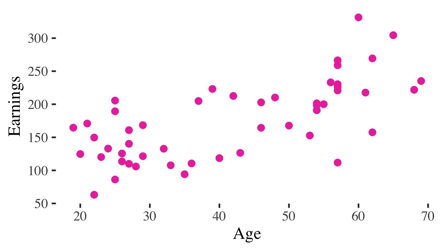
Both correlation and regression are based on a description of a line used to characterize data points in a scatterplot
Correlation vs. bivariate regression
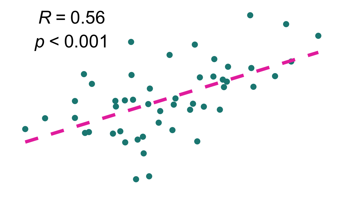
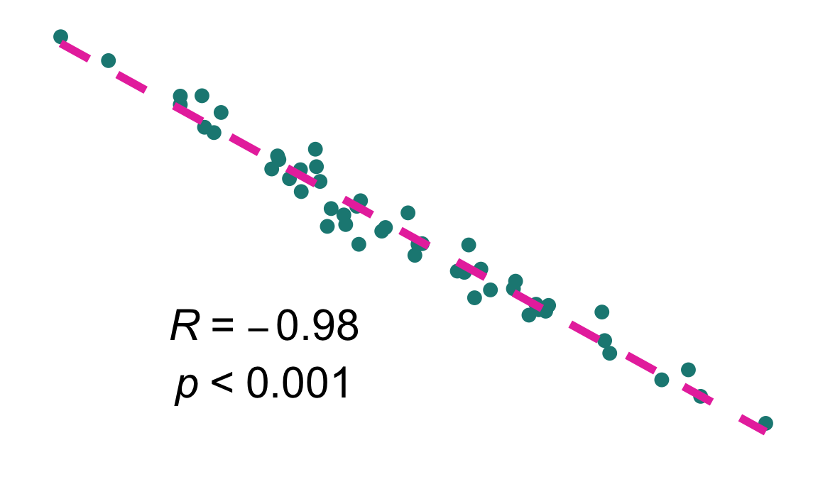
Correlation:
- assess how tightly clustered points in the scatterplot around a line
Bivariate Regression:
- describe the line that characterizes the points in the scatterplot
- tells us how the dependent (Y) variable changes for a one-unit change in the independent (X) variable
- allows us to predict values of Y based on values of X
Examples of questions bivariate regression can help us answer:
- What kind of GPA would we predict for someone who studies for 15 hours per week?
- Based on the data, how many dates would we predict for a person with a GPA of 3.5?
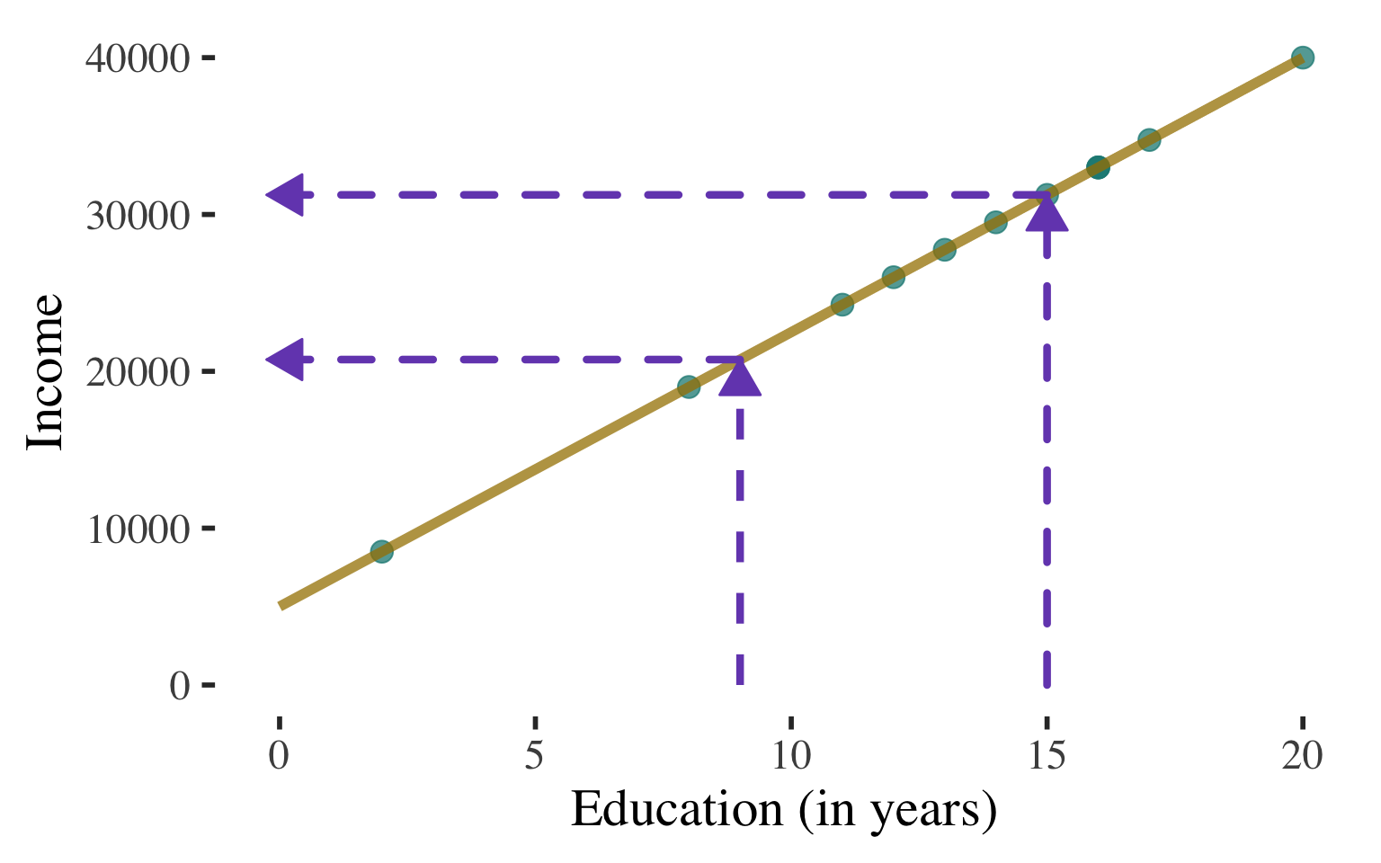
- If someone has 16 years of education, what is our best prediction of their income?
Bivariate Regression
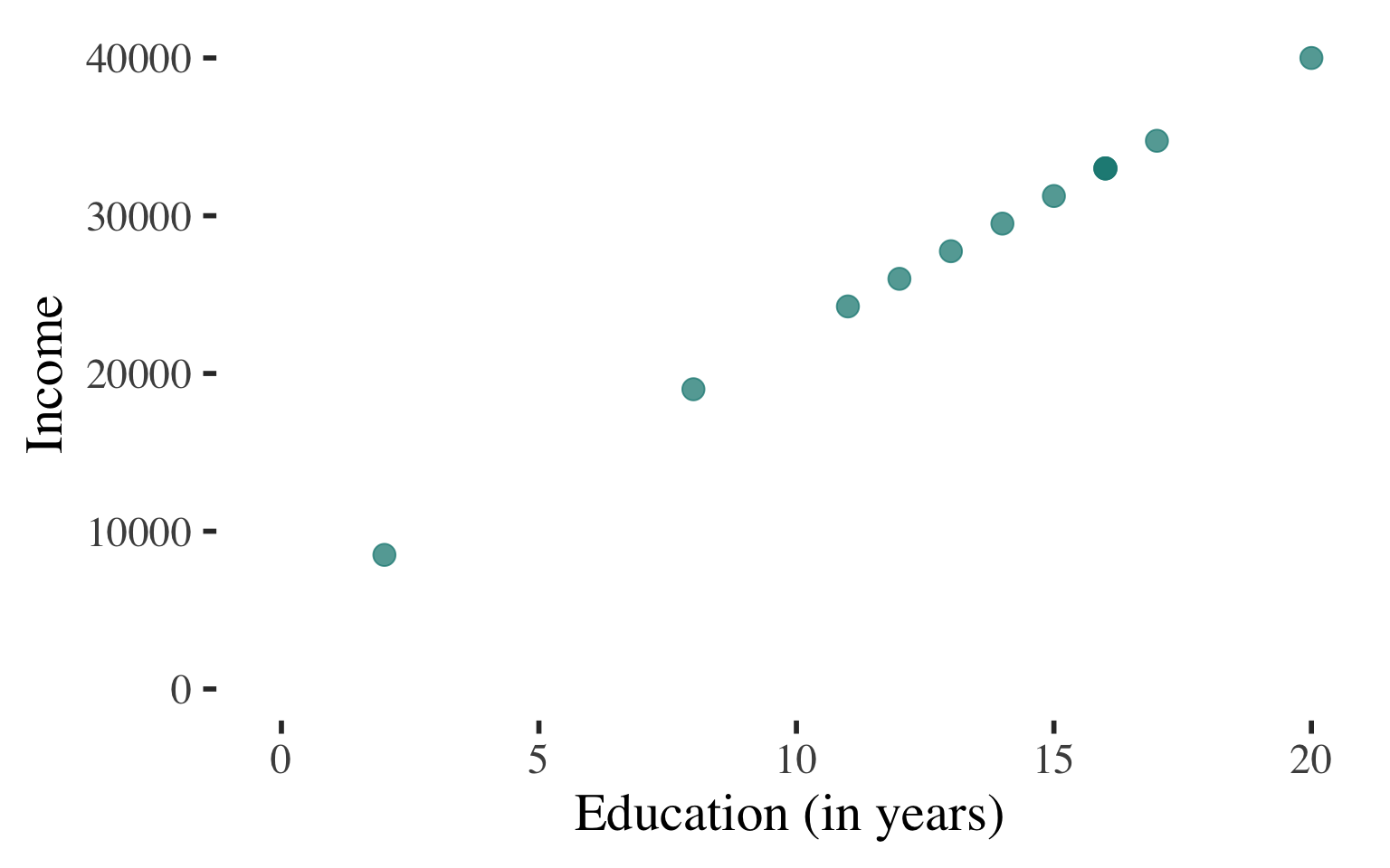
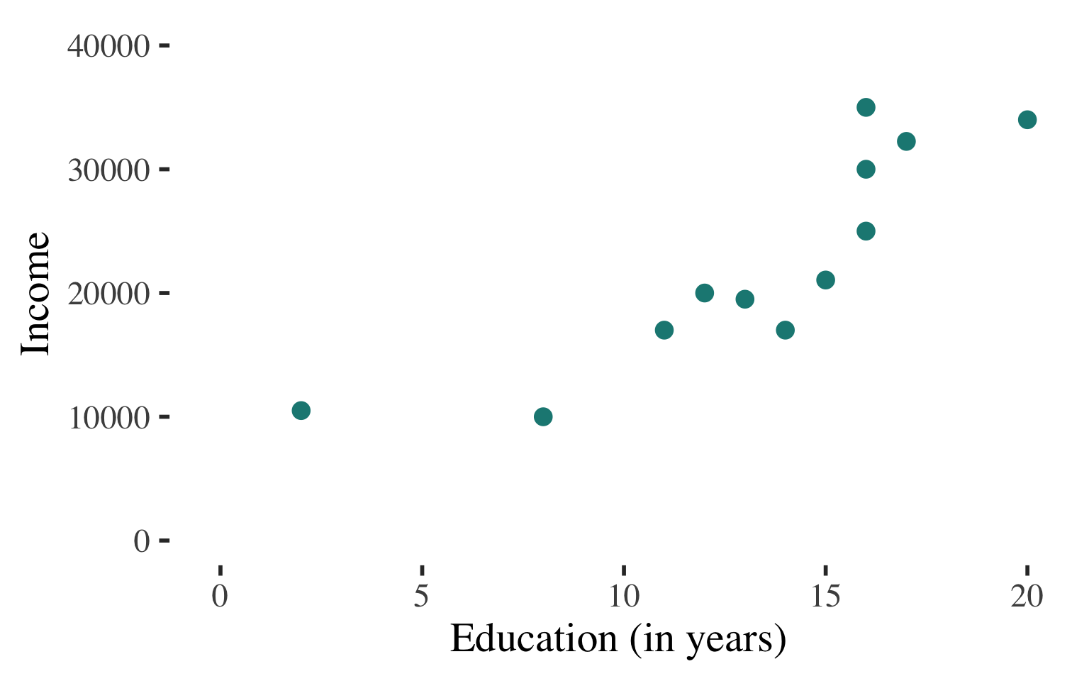
Draw a scatterplot
Use a line to describe the
pattern of points
| Education | Income |
|---|---|
| 12 | 26000 |
| 16 | 33000 |
| 13 | 27750 |
| 14 | 29500 |
| 8 | 19000 |
| 15 | 31250 |
| 16 | 33000 |
| 16 | 33000 |
| 11 | 24250 |
| 20 | 40000 |
| 17 | 34750 |
| 2 | 8500 |
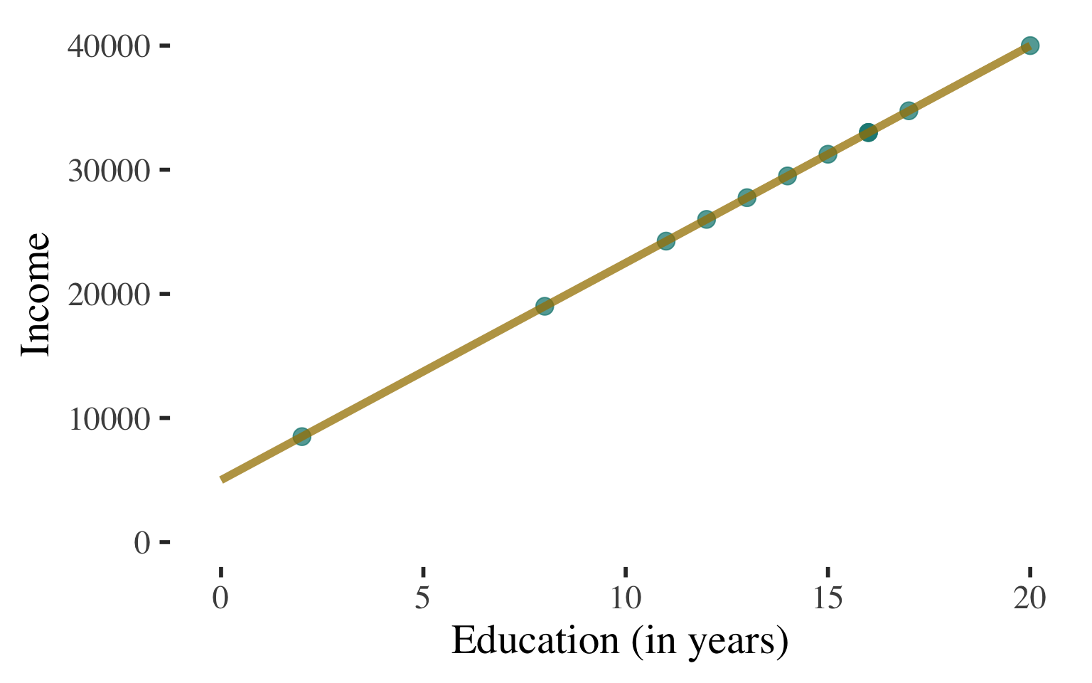
Can use this line to predict the level of income for a person with any level of education
(within the range that we observe)
Bivariate Regression
\(\widehat{y}\) \(=\) \(a\) \(+\) \(b\)\(x\)
Describe the line to describe the association and predict values of the dependent variable
Blah

Bivariate Regression
\(\widehat{y}\) \(=\) \(a\) \(+\) \(b\)\(x\)
\(\widehat{y}\) is the predicted value of \(Y\)
(the dependent variable)
Describe the line to describe the association and predict values of the dependent variable
Blah

Bivariate Regression
\(\widehat{y}\) \(=\) \(a\) \(+\) \(b\)\(x\)
\(\widehat{y}\) is the predicted value of \(Y\)
(the dependent variable)
\(x\) is the value of \(X\)
for the individual
Describe the line to describe the association and predict values of the dependent variable
Blah

Bivariate Regression
\(\widehat{y}\) \(=\) \(a\) \(+\) \(b\)\(x\)
\(\widehat{y}\) is the predicted value of \(Y\)
(the dependent variable)
\(x\) is the value of \(X\)
for the individual
\(b = \text{slope of the line}\)
(i.e. how much \(Y\) changes with each one-unit difference in \(X\))
Describe the line to describe the association and predict values of the dependent variable
Blah

Bivariate Regression
\(\widehat{y}\) \(=\) \(a\) \(+\) \(b\)\(x\)
\(\widehat{y}\) is the predicted value of \(Y\)
(the dependent variable)
\(x\) is the value of \(X\)
for the individual
\(b = \text{slope of the line}\)
(i.e. how much \(Y\) changes with each one-unit difference in \(X\))
\(a = \text{Y-intercept}\)
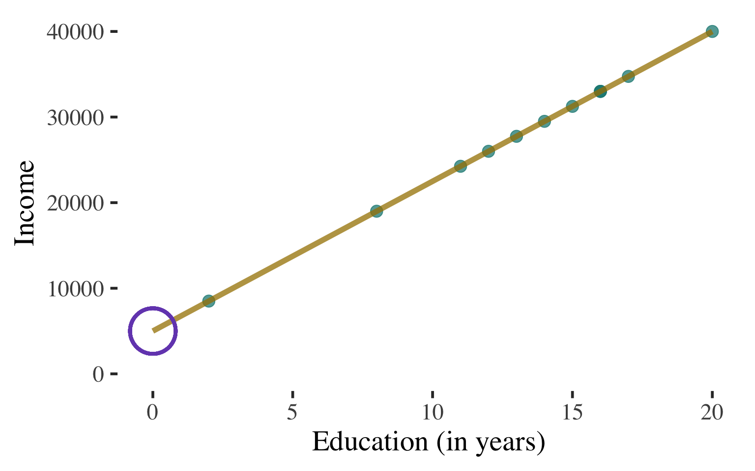
(the predicted value of \(Y\) when \(X = 0\); a.k.a. the constant)
Describe the line to describe the association and predict values of the dependent variable
Blah
Bivariate Regression
\(\widehat{y}\) \(=\) \(a\) \(+\) \(b\)\(x\)
\(\widehat{y}\) \(=\) \(5000\) \(+\) \(1750\)\(x\)
Describe the line to describe the association and predict values of the dependent variable
Blah

Bivariate Regression
\(\widehat{y}\) \(=\) \(a\) \(+\) \(b\)\(x\)
\(\widehat{y}\) \(=\) \(5000\) \(+\) \(1750\)\(x\)
A person with \(0\) years of education is predicted to make \(\$5,000\)
Describe the line to describe the association and predict values of the dependent variable
Blah
Bivariate Regression
\(\widehat{y}\) \(=\) \(a\) \(+\) \(b\)\(x\)
\(\widehat{y}\) \(=\) \(5000\) \(+\) \(1750\)\(x\)
A person with \(0\) years of education is predicted to make \(\$5,000\)
Describe the line to describe the association and predict values of the dependent variable
Blah
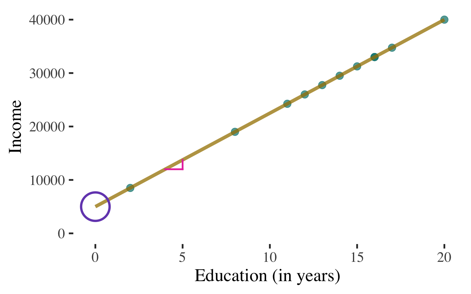
Income is predicted to increase by \(\$1,750\) for each additional year of education
Bivariate Regression
\(\widehat{y}\) \(=\) \(5000\) \(+\) \(1750\)\(x\)
Deterministic association:
All of the points in the scatterplot fall on the line.
Perfectly predict
\(Y\) based on \(X\).
\(|r| = 1.0\)
Describe the line to describe the association and predict values of the dependent variable
Blah

Bivariate Regression
\(\widehat{y}\) \(=\) \(a\) \(+\) \(b\)\(x\)
Non-deterministic association:
Points in the scatterplot do not all fall on the line
Cannot perfectly predict \(Y\) based on \(X\).
\(|r| \lt 1.0\)
Describe the line to describe the association and predict values of the dependent variable
Blah

Bivariate Regression
\(\widehat{y}\) \(=\) \(a\) \(+\) \(b\)\(x\)
Non-deterministic association:
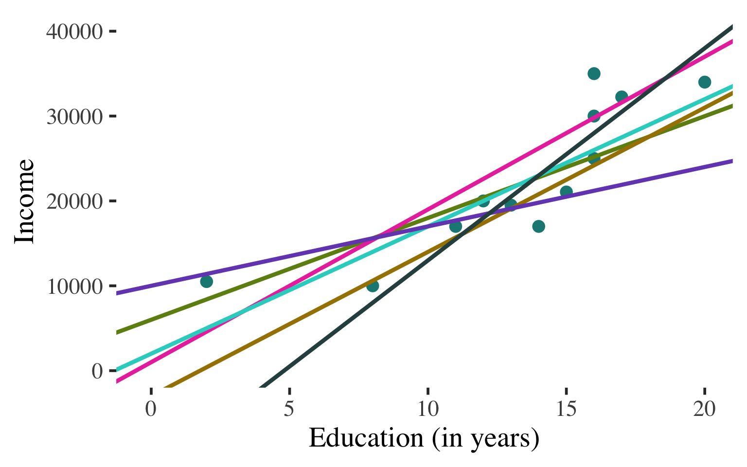
A lot of different lines appear to characterize the points
Each line comes close to some points but misses others by a lot.
Describe the line to describe the association and predict values of the dependent variable
Blah

Bivariate Regression
\(\widehat{y}\) \(=\) \(a\) \(+\) \(b\)\(x\)
Want the line that fits the data best - i.e. comes as close as possible, on average, to all points
Technically: Want the line that minimizes the (squared) errors we would make in predicting \(Y\) with the line
Looking for the least squares regression line
Describe the line to describe the association and predict values of the dependent variable
Blah
Bivariate Regression
\(\widehat{y}\) \(=\) \(a\) \(+\) \(b\)\(x\)
Want the line that fits the data best - i.e. comes as close as possible, on average, to all points
Need two components of the regression line:
- \(a\) (y-intercept)
- \(b\) (slope)
Calculating the least squares regression line
Step 1: calculate the slope
\[\begin{aligned} \color{#e93cac}{b} = {r}(\frac{{s_y}}{{s_x}}) \end{aligned}\]
Bivariate Regression
\(\widehat{y}\) \(=\) \(a\) \(+\) \(b\)\(x\)
Want the line that fits the data best - i.e. comes as close as possible, on average, to all points
Need two components of the regression line:
- \(a\) (y-intercept)
- \(b\) (slope)
Calculating the least squares regression line
Step 1: calculate the slope
\[\begin{aligned} \color{#e93cac}{b} = \color{#a68100}{r}(\frac{{s_y}}{{s_x}}) \end{aligned}\]
Correlation coefficient
Bivariate Regression
\(\widehat{y}\) \(=\) \(a\) \(+\) \(b\)\(x\)
Want the line that fits the data best - i.e. comes as close as possible, on average, to all points
Need two components of the regression line:
- \(a\) (y-intercept)
- \(b\) (slope)
Calculating the least squares regression line
Step 1: calculate the slope
\[\begin{aligned} \color{#e93cac}{b} = \color{#a68100}{r}(\frac{\color{#6e8e13}{s_y}}{{s_x}}) \end{aligned}\]
Correlation coefficient
Standard deviation of
the dependent variable
Bivariate Regression
\(\widehat{y}\) \(=\) \(a\) \(+\) \(b\)\(x\)
Want the line that fits the data best - i.e. comes as close as possible, on average, to all points
Need two components of the regression line:
- \(a\) (y-intercept)
- \(b\) (slope)
Calculating the least squares regression line
Step 1: calculate the slope
\[\begin{aligned} \color{#e93cac}{b} = \color{#a68100}{r}(\frac{\color{#6e8e13}{s_y}}{\color{#1b8883}{s_x}}) \end{aligned}\]
Correlation coefficient
Standard deviation of
the dependent variable
Standard deviation of
the independent variable
Bivariate Regression
\(\widehat{y}\) \(=\) \(a\) \(+\) \(b\)\(x\)
Want the line that fits the data best - i.e. comes as close as possible, on average, to all points
Need two components of the regression line:
- \(a\) (y-intercept)
- \(b\) (slope)
Calculating the least squares regression line
Step 2: calculate the Y-intercept
\[\begin{aligned} \color{#754cbc}{a} = \color{#6e8e13}{\bar{y}}-\color{#e93cac}{b}\color{#1b8883}{\bar{x}} \end{aligned}\]
Mean of the
dependent variable
Slope
Mean of the
independent variable
Bivariate Regression
Step 1: calculate the slope
\[\begin{aligned} \color{#e93cac}b &= r(\frac{s_y}{s_x}) \\ &= 0.857(\frac{8655.131}{4.735}) \\ &= \color{#e93cac}{1566.515} \end{aligned}\]
Income increases by \(\color{#e93cac}{\$1,566.52}\) for each additional year of education
\(\bar{y} =\) 22608.333 \(\bar{x} =\) 13.333
\(s_y =\) 8655.131 \(s_x =\) 4.735
\(r =\) 0.857

Bivariate Regression
Step 2: calculate the Y-intercept
\[\begin{aligned} \color{#754cbc}a &= \bar{y} - b\bar{x} \\ &= 22608.333 - (1566.515)(13.333) \\ &= \color{#754cbc}{1721.989} \end{aligned}\]
A person with \(0\) years of
education is predicted to
make \(\color{#754cbc}{\$1721.99}\).
\(\bar{y} =\) 22608.333 \(\bar{x} =\) 13.333
\(s_y =\) 8655.131 \(s_x =\) 4.735
\(r =\) 0.857
Bivariate Regression
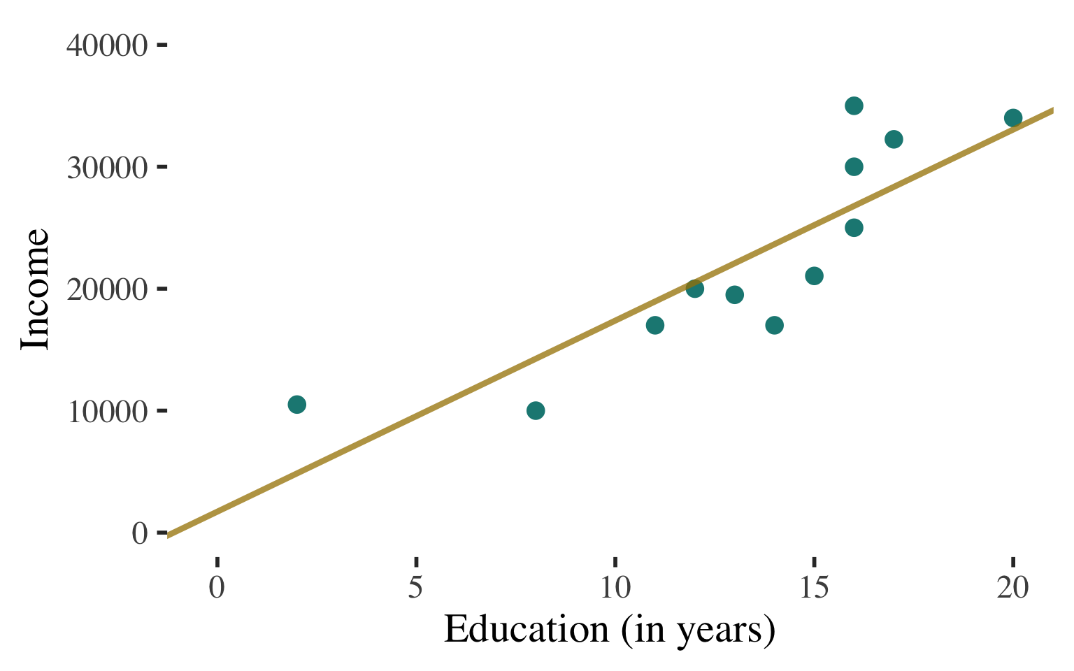
Ordinary least squares regression line: \(\widehat{y} = a + bx\)
\(\widehat{\text{Income}} = 1721.989 + 1566.515(\text{Education})\)
This is the line that fits the data best - i.e., comes as close as possible, on average, to all points.
Technically: The line that minimizes the (squared) errors we would make in predicting Y with the line
Bivariate Regression
Ordinary least squares regression line: \(\widehat{y} = a + bx\)
\(\widehat{\text{Income}} = 1721.989 + 1566.515(\text{Education})\)
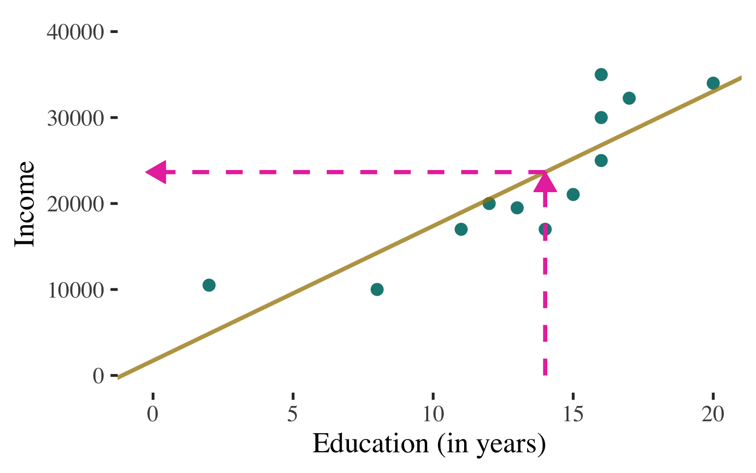
Can use this line to predict values of Y (income) for any value of X (education)
Example: What is the predicted level of income for a person with 14 years of education?
\(\begin{aligned} \widehat{\text{Income}} &= 1721.989 + 1566.515(14) \\ &= 23653.20 \end{aligned}\)
How well does the best fitting line fit the data?
Coefficient of Determination
Assessing the fit of the regression line
\(\widehat{\text{Income}} = 1721.989 + 1566.515(\text{Education})\)
This is the line that fits the data best - i.e., comes as close as possible, on average, to all points.
BUT STILL DOES NOT “FIT”
THE DATA PERFECTLY
(misses some points)

Coefficient of Determination
Assessing the fit of the regression line
\(\widehat{\text{Income}} = 1721.989 + 1566.515(\text{Education})\)
Coefficient of determination (\(R^2\)) measures the level of model fit
\[ R^2 = (\color{#1b8883}{r})(\color{#1b8883}{r}) \]
Simply square the
correlation coefficient
Range of \(R^2\):
\(0.0 =\) no association,
no predictive value of knowing X
\(1.0 =\) deterministic

Interpretation of the Coefficient of Determination
\[ R^2 = (r)(r) \]
INTERPRETATION #1

Interpretation of the Coefficient of Determination
\[ R^2 = (r)(r) \]
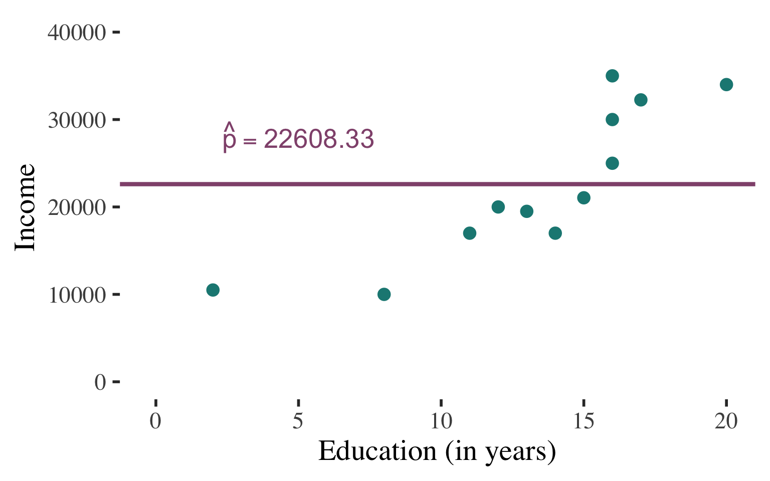
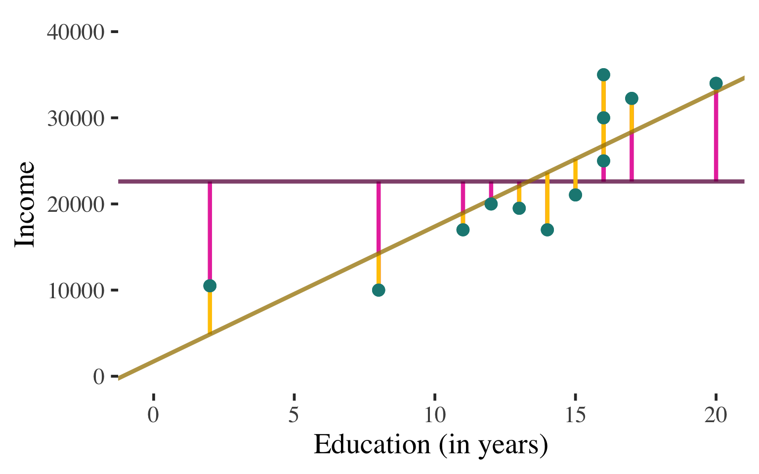
In the absence of any other information, we would just guess the mean for the income of any individual (since the mean is the balancing point of the distribution)
INTERPRETATION #1
Interpretation of the Coefficient of Determination
\[ R^2 = (r)(r) \]
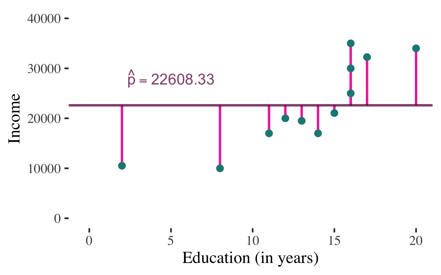
In the absence of any other information, we would just guess the mean for the income of any individual (since the mean is the balancing point of the distribution)
For almost all cases there would be ERROR in these predictions
\(y \ne \bar{y}\)
INTERPRETATION #1
Interpretation of the Coefficient of Determination
\[ R^2 = (r)(r) \]
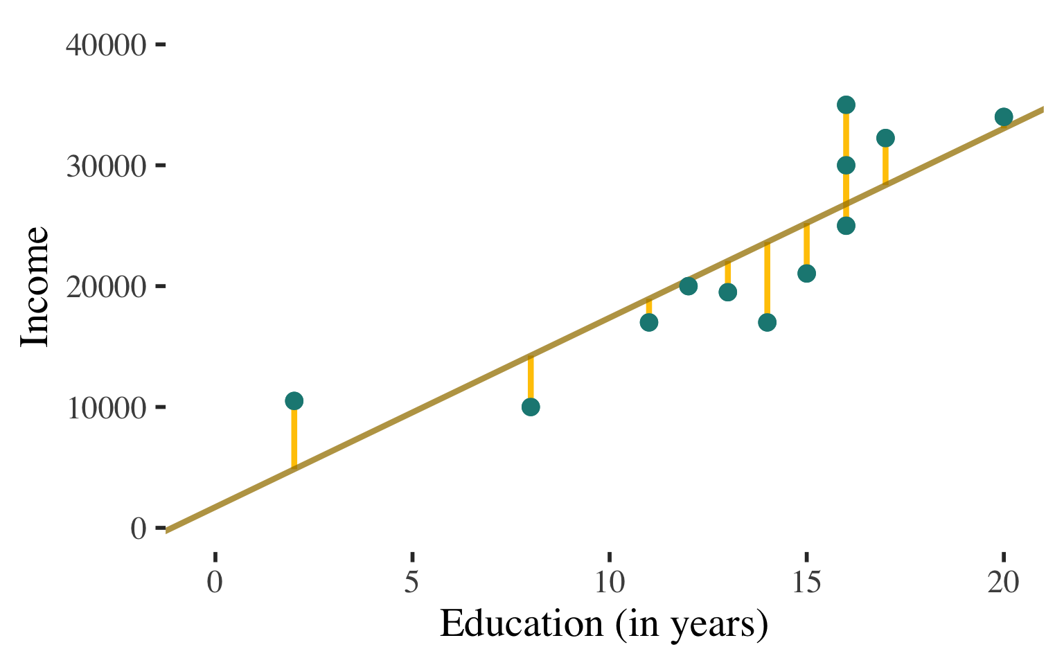
If we know individuals’ level of education, we would use this information to predict individual income (regression line represents the best prediction line for the association between education and income)
INTERPRETATION #1

Interpretation of the Coefficient of Determination
\[ R^2 = (r)(r) \]
If we know individuals’ level of education, we would use this information to predict individual income (regression line represents the best prediction line for the association between education and income)
For almost all cases there would be ERROR in these predictions
\(y \ne \widehat{y}\)
INTERPRETATION #1
Interpretation of the Coefficient of Determination
\[ R^2 = (r)(r) \]
QUESTION:
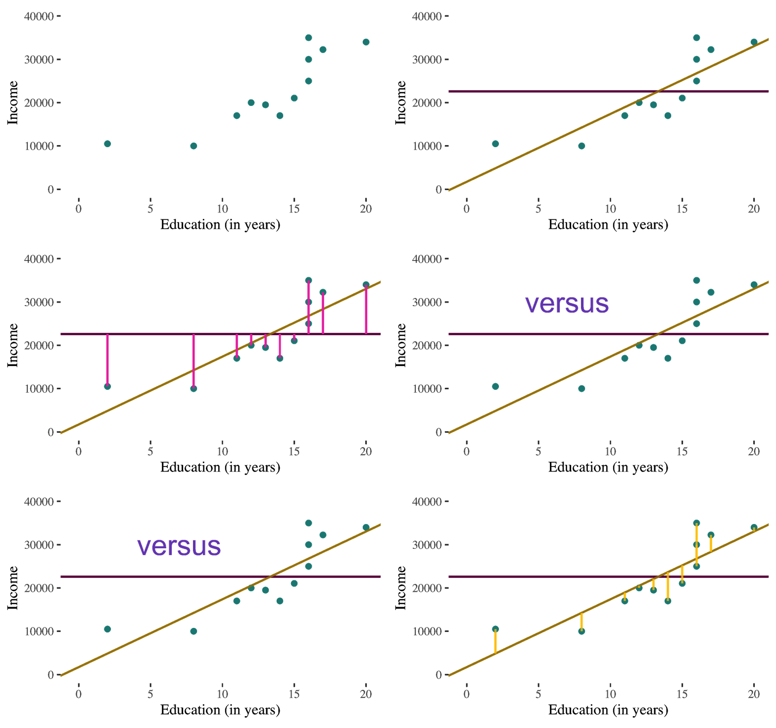
How much better do we do in predicting the dependent variable using the regression line versus just guessing the mean value?
\(\begin{aligned}r &= 0.857 \\ R^2 &= (r)(r) \\ &= (0.857)(0.857) \\&= 0.734 \end{aligned}\)
INTERPRETATION #1
Interpretation of the Coefficient of Determination
\[ R^2 = (r)(r) \]
If we are predicting individuals’ income, we will reduce our errors of prediction by about 73% if we take into consideration how much education these individuals have.
\(\begin{aligned}r &= 0.857 \\ R^2 &= (r)(r) \\ &= (0.857)(0.857) \\&= 0.734 \end{aligned}\)
INTERPRETATION #1
The proportional reduction of prediction error achieved by using the linear regression equation to predict the values of the dependent variable (Y)
Interpretation of the Coefficient of Determination
\[ R^2 = (r)(r) \]
INTERPRETATION #2

Interpretation of the Coefficient of Determination
\[ R^2 = (r)(r) \]
QUESTION:
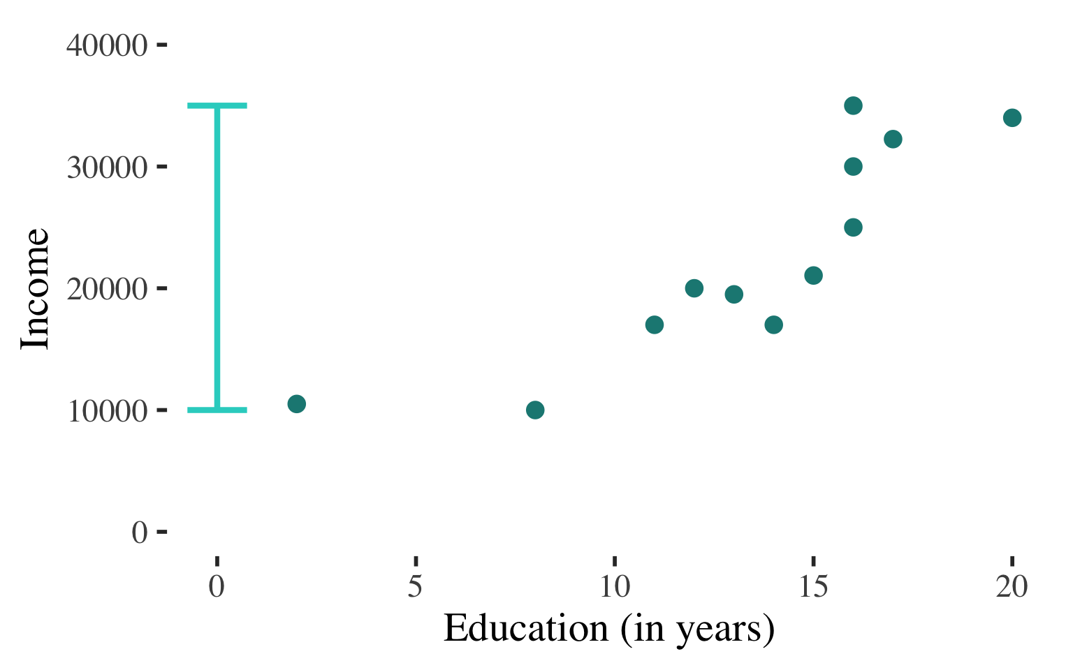
How much of this variation is due to the fact that people have different levels of education?
Income varies!
\(\begin{aligned}r &= 0.857 \\ R^2 &= (r)(r) \\ &= (0.857)(0.857) \\&= 0.734 \end{aligned}\)
INTERPRETATION #2
The proportion of the variance in the dependent variable (\(Y\)) explained by the independent variable (\(X\))
Interpretation of the Coefficient of Determination
\[ R^2 = (r)(r) \]
About \(73\%\) of the variation in income is explained by the diversity of education levels in the sample.
Income varies!
\(\begin{aligned}r &= 0.857 \\ R^2 &= (r)(r) \\ &= (0.857)(0.857) \\&= 0.734 \end{aligned}\)
INTERPRETATION #2
The proportion of the variance in the dependent variable (\(Y\)) explained by the independent variable (\(X\))

Break!
Practice
A researcher collected the following data on years of education (\(X\)) and number of children (\(Y\)) for a sample of married adults and produced the following raw data.
| Education (\(x_i\)) | # Kids (\(y_i\)) | \(x_i -\bar{x}\) | \(\frac{x_i-\bar{x}}{s_x}\) | \(y_i -\bar{y}\) | \(\frac{y_i-\bar{y}}{s_y}\) | \((\frac{x_i-\bar{x}}{s_x})(\frac{y_i-\bar{y}}{s_y})\) | |
|---|---|---|---|---|---|---|---|
| 12 | 2 | -1.00 | -0.29 | -0.20 | -0.12 | 0.04 | |
| 14 | 1 | 1.00 | 0.29 | -1.20 | -0.74 | -0.22 | |
| 17 | 0 | 4.00 | 1.18 | -2.20 | -1.36 | -1.60 | |
| 10 | 3 | -3.00 | -0.88 | 0.80 | 0.49 | -0.44 | |
| 8 | 5 | -5.00 | -1.47 | 2.80 | 1.73 | -2.54 | |
| 9 | 3 | -4.00 | -1.18 | 0.80 | 0.49 | -0.58 | |
| 12 | 4 | -1.00 | -0.29 | 1.80 | 1.11 | -0.33 | |
| 14 | 2 | 1.00 | 0.29 | -0.20 | -0.12 | -0.04 | |
| 18 | 0 | 5.00 | 1.47 | -2.20 | -1.36 | -2.00 | |
| 16 | 2 | 3.00 | 0.88 | -0.20 | -0.12 | -0.11 | |
| sum | 130 | 22 | |||||
| mean | 13 | 2.2 | |||||
| st. dev. | 3.399 | 1.619 |
- Calculate the correlation between education and number of kids
- Find the OLS regression line for the effect of education on number of kids
- What is the prediction error for the first person in the data set?
- Find and interpret the coefficient of determination
A researcher collected the following data on years of education (\(X\)) and number of children (\(Y\)) for a sample of married adults and produced the following raw data.
| Education (\(x_i\)) | # Kids (\(y_i\)) | \(x_i -\bar{x}\) | \(\frac{x_i-\bar{x}}{s_x}\) | \(y_i -\bar{y}\) | \(\frac{y_i-\bar{y}}{s_y}\) | \((\frac{x_i-\bar{x}}{s_x})(\frac{y_i-\bar{y}}{s_y})\) | |
|---|---|---|---|---|---|---|---|
| 12 | 2 | -1.00 | -0.29 | -0.20 | -0.12 | 0.04 | |
| 14 | 1 | 1.00 | 0.29 | -1.20 | -0.74 | -0.22 | |
| 17 | 0 | 4.00 | 1.18 | -2.20 | -1.36 | -1.60 | |
| 10 | 3 | -3.00 | -0.88 | 0.80 | 0.49 | -0.44 | |
| 8 | 5 | -5.00 | -1.47 | 2.80 | 1.73 | -2.54 | |
| 9 | 3 | -4.00 | -1.18 | 0.80 | 0.49 | -0.58 | |
| 12 | 4 | -1.00 | -0.29 | 1.80 | 1.11 | -0.33 | |
| 14 | 2 | 1.00 | 0.29 | -0.20 | -0.12 | -0.04 | |
| 18 | 0 | 5.00 | 1.47 | -2.20 | -1.36 | -2.00 | |
| 16 | 2 | 3.00 | 0.88 | -0.20 | -0.12 | -0.11 | |
| sum | 130 | 22 | -7.81 | ||||
| mean | 13 | 2.2 | |||||
| st. dev. | 3.399 | 1.619 | \(r =\) | \(-0.868\) |
- Find the OLS regression line for the effect of education on number of kids
\[ \widehat{y} = a + bx \]
\[ \begin{aligned} \color{#e93cac}b &= \color{#a68100}r(\frac{\color{#6e8e13}{s_y}}{\color{#1b8883}{s_x}}) \\ &= (\color{#a68100}{-0.868})(\frac{\color{#6e8e13}{1.619}}{\color{#1b8883}{3.399}}) \\ &= \color{#e93cac}{-0.413} \end{aligned} \]
A researcher collected the following data on years of education (\(X\)) and number of children (\(Y\)) for a sample of married adults and produced the following raw data.
| Education (\(x_i\)) | # Kids (\(y_i\)) | \(x_i -\bar{x}\) | \(\frac{x_i-\bar{x}}{s_x}\) | \(y_i -\bar{y}\) | \(\frac{y_i-\bar{y}}{s_y}\) | \((\frac{x_i-\bar{x}}{s_x})(\frac{y_i-\bar{y}}{s_y})\) | |
|---|---|---|---|---|---|---|---|
| 12 | 2 | -1.00 | -0.29 | -0.20 | -0.12 | 0.04 | |
| 14 | 1 | 1.00 | 0.29 | -1.20 | -0.74 | -0.22 | |
| 17 | 0 | 4.00 | 1.18 | -2.20 | -1.36 | -1.60 | |
| 10 | 3 | -3.00 | -0.88 | 0.80 | 0.49 | -0.44 | |
| 8 | 5 | -5.00 | -1.47 | 2.80 | 1.73 | -2.54 | |
| 9 | 3 | -4.00 | -1.18 | 0.80 | 0.49 | -0.58 | |
| 12 | 4 | -1.00 | -0.29 | 1.80 | 1.11 | -0.33 | |
| 14 | 2 | 1.00 | 0.29 | -0.20 | -0.12 | -0.04 | |
| 18 | 0 | 5.00 | 1.47 | -2.20 | -1.36 | -2.00 | |
| 16 | 2 | 3.00 | 0.88 | -0.20 | -0.12 | -0.11 | |
| sum | 130 | 22 | -7.81 | ||||
| mean | 13 | 2.2 | |||||
| st. dev. | 3.399 | 1.619 | \(r =\) | \(-0.868\) |
- Find the OLS regression line for the effect of education on number of kids
\[ \widehat{y} = a + bx \]
\[ \begin{aligned} \color{#754cbc}a &= \color{#6e8e13}{\bar{y}}- \color{#e93cac}{b}\color{#1b8883}{\bar{x}} \\ &= \color{#6e8e13}{2.20} - (\color{#e93cac}{-0.413})(\color{#1b8883}{13.00}) \\ &= \color{#754cbc}{7.569} \end{aligned} \]
A researcher collected the following data on years of education (\(X\)) and number of children (\(Y\)) for a sample of married adults and produced the following raw data.
| Education (\(x_i\)) | # Kids (\(y_i\)) | \(x_i -\bar{x}\) | \(\frac{x_i-\bar{x}}{s_x}\) | \(y_i -\bar{y}\) | \(\frac{y_i-\bar{y}}{s_y}\) | \((\frac{x_i-\bar{x}}{s_x})(\frac{y_i-\bar{y}}{s_y})\) | |
|---|---|---|---|---|---|---|---|
| 12 | 2 | -1.00 | -0.29 | -0.20 | -0.12 | 0.04 | |
| 14 | 1 | 1.00 | 0.29 | -1.20 | -0.74 | -0.22 | |
| 17 | 0 | 4.00 | 1.18 | -2.20 | -1.36 | -1.60 | |
| 10 | 3 | -3.00 | -0.88 | 0.80 | 0.49 | -0.44 | |
| 8 | 5 | -5.00 | -1.47 | 2.80 | 1.73 | -2.54 | |
| 9 | 3 | -4.00 | -1.18 | 0.80 | 0.49 | -0.58 | |
| 12 | 4 | -1.00 | -0.29 | 1.80 | 1.11 | -0.33 | |
| 14 | 2 | 1.00 | 0.29 | -0.20 | -0.12 | -0.04 | |
| 18 | 0 | 5.00 | 1.47 | -2.20 | -1.36 | -2.00 | |
| 16 | 2 | 3.00 | 0.88 | -0.20 | -0.12 | -0.11 | |
| sum | 130 | 22 | -7.81 | ||||
| mean | 13 | 2.2 | |||||
| st. dev. | 3.399 | 1.619 | \(r =\) | \(-0.868\) |
- Find the OLS regression line for the effect of education on number of kids
\[ \widehat{y} = a + bx \]
\[ \widehat{y} = 7.569 - 0.413x \]
A researcher collected the following data on years of education (\(X\)) and number of children (\(Y\)) for a sample of married adults and produced the following raw data.
| Education (\(x_i\)) | # Kids (\(y_i\)) | \(x_i -\bar{x}\) | \(\frac{x_i-\bar{x}}{s_x}\) | \(y_i -\bar{y}\) | \(\frac{y_i-\bar{y}}{s_y}\) | \((\frac{x_i-\bar{x}}{s_x})(\frac{y_i-\bar{y}}{s_y})\) | |
|---|---|---|---|---|---|---|---|
| 12 | 2 | -1.00 | -0.29 | -0.20 | -0.12 | 0.04 | |
| 14 | 1 | 1.00 | 0.29 | -1.20 | -0.74 | -0.22 | |
| 17 | 0 | 4.00 | 1.18 | -2.20 | -1.36 | -1.60 | |
| 10 | 3 | -3.00 | -0.88 | 0.80 | 0.49 | -0.44 | |
| 8 | 5 | -5.00 | -1.47 | 2.80 | 1.73 | -2.54 | |
| 9 | 3 | -4.00 | -1.18 | 0.80 | 0.49 | -0.58 | |
| 12 | 4 | -1.00 | -0.29 | 1.80 | 1.11 | -0.33 | |
| 14 | 2 | 1.00 | 0.29 | -0.20 | -0.12 | -0.04 | |
| 18 | 0 | 5.00 | 1.47 | -2.20 | -1.36 | -2.00 | |
| 16 | 2 | 3.00 | 0.88 | -0.20 | -0.12 | -0.11 | |
| sum | 130 | 22 | -7.81 | ||||
| mean | 13 | 2.2 | |||||
| st. dev. | 3.399 | 1.619 | \(r =\) | \(-0.868\) |
- What is the prediction error for the first person in the data set?
\[ \widehat{y} = 7.569 - 0.413x \]
\[ \widehat{y} = a + bx \]
\[ \text{prediction error} = y - \widehat{y} \]
\[ \begin{aligned} \color{#a68100}{\widehat{Kids_1}} &= 7.569 - 0.413(\color{#1b8883}{12}) \\ &= \color{#a68100}{2.613} \end{aligned} \]
\[ \begin{aligned} \text{prediction error} &= \color{#754cbc}{2} - \color{#a68100}{2.613} \\ &= -0.613 \end{aligned} \]
A researcher collected the following data on years of education (\(X\)) and number of children (\(Y\)) for a sample of married adults and produced the following raw data.
| Education (\(x_i\)) | # Kids (\(y_i\)) | \(x_i -\bar{x}\) | \(\frac{x_i-\bar{x}}{s_x}\) | \(y_i -\bar{y}\) | \(\frac{y_i-\bar{y}}{s_y}\) | \((\frac{x_i-\bar{x}}{s_x})(\frac{y_i-\bar{y}}{s_y})\) | |
|---|---|---|---|---|---|---|---|
| 12 | 2 | -1.00 | -0.29 | -0.20 | -0.12 | 0.04 | |
| 14 | 1 | 1.00 | 0.29 | -1.20 | -0.74 | -0.22 | |
| 17 | 0 | 4.00 | 1.18 | -2.20 | -1.36 | -1.60 | |
| 10 | 3 | -3.00 | -0.88 | 0.80 | 0.49 | -0.44 | |
| 8 | 5 | -5.00 | -1.47 | 2.80 | 1.73 | -2.54 | |
| 9 | 3 | -4.00 | -1.18 | 0.80 | 0.49 | -0.58 | |
| 12 | 4 | -1.00 | -0.29 | 1.80 | 1.11 | -0.33 | |
| 14 | 2 | 1.00 | 0.29 | -0.20 | -0.12 | -0.04 | |
| 18 | 0 | 5.00 | 1.47 | -2.20 | -1.36 | -2.00 | |
| 16 | 2 | 3.00 | 0.88 | -0.20 | -0.12 | -0.11 | |
| sum | 130 | 22 | -7.81 | ||||
| mean | 13 | 2.2 | |||||
| st. dev. | 3.399 | 1.619 | \(r =\) | \(-0.868\) |
- Find and interpret the coefficient of determination
\[ \begin{aligned} \color{#a68100}{r} &= \color{#a68100}{-0.868} \\ R^2 &= (\color{#a68100}{r})(\color{#a68100}{r}) \\ &= (\color{#a68100}{-0.868})(\color{#a68100}{-0.868}) \\ &= 0.753 \end{aligned} \]
If we are predicting the number of kids individuals have, we will reduce our errors of prediction by about \(75\%\) if we take into consideration how much education these individuals have.
About \(75\%\) of the variation in number of kids is explained by the diversity of education levels in the sample.
Statistical significance of regression componenets
STATISTICAL SIGNIFICANCE
How certain can we be that the association exists in the population?
\[ \widehat{y} = a + bx \]
Rarely interested in statistical significance of the Y-intercept (whether the starting point of the line is different from \(0\) in the population)
There IS usually interest in whether the slope is statistically significant (whether the change in the dependent variable associated with a one-unit change in the independent variable is different from \(0\) in the population)
If \(r\) is statistically significant then the bivariate slope is also statistically significant at the same alpha level.