Writing Functions

CS&SS 508 • Lecture 8

14 May 2024

Victoria Sass

Roadmap

Last time, we learned:

• Types of Data
  • Strings
• Pattern Matching & Regular Expressions

Today, we will cover:

• Function Basics
• Types of Functions
  • Vector Functions
  • Dataframe Functions
  • Plot Functions
• Function Style Guide

Function Basics

Why Functions?

R (as well as mathematics in general) is full of functions!

We use functions to:

• Compute summary statistics (mean(), sd(), min())
• Fit models to data (lm(Fertility ~ Agriculture, data = swiss))
• Read in data (read_csv())
• Create visualizations (ggplot())
• And a lot more!!

Examples of Existing Functions

• mean():
  • Input: a vector
  • Output: a single number
• dplyr::filter():
  • Input: a data frame, logical conditions
  • Output: a data frame with rows removed using those conditions
• readr::read_csv():
  • Input: a file path, optionally variable names or types
  • Output: a data frame containing info read in from file

Each function requires inputs, and returns outputs

Why Write Your Own Functions?

• Functions allow you to automate common tasks in a more powerful and general way than copy-and-pasting
• As requirements change, you only need to update code in one place, instead of many.
• You eliminate the chance of making incidental mistakes compared to when you copy and paste (i.e. updating a variable name in one place, but not in another).
• It makes it easier to reuse work from project-to-project, increasing your productivity over time.
• If well named, your function can make your overall code easier to understand.

Plan your Function before Writing

Before you can write effective code, you need to know exactly what you want:

• Goal: Do I want a single value? vector? one observation per person? per year?
• Current State: What do I currently have? data frame, vector? long or wide format?
• Translate: How can I take what I have and turn it into my goal?
  • Sketch out the steps!
  • Break it down into little operations

As we become more advanced coders, this concept is key!!

Remember: When you’re stuck, try searching your problem on Google!!

Simple, Motivating Example

df <- tibble(
  a = rnorm(5),
  b = rnorm(5),
  c = rnorm(5),
  d = rnorm(5)
  )
df

df |> mutate(
  a = (a - min(a, na.rm = TRUE)) / 
    (max(a, na.rm = TRUE) - min(a, na.rm = TRUE)),
  b = (b - min(b, na.rm = TRUE)) / 
    (max(b, na.rm = TRUE) - min(a, na.rm = TRUE)),
  c = (c - min(c, na.rm = TRUE)) / 
    (max(c, na.rm = TRUE) - min(c, na.rm = TRUE)),
  d = (d - min(d, na.rm = TRUE)) / 
    (max(d, na.rm = TRUE) - min(d, na.rm = TRUE))
  )

• What do you think this code does?
• Are there any typos?
• Could we write this more efficiently as a function?

> # A tibble: 5 × 4
>        a       b      c      d
>    <dbl>   <dbl>  <dbl>  <dbl>
> 1 -0.130 -0.398   0.347  0.368
> 2 -1.14   1.04   -0.433 -1.07 
> 3 -2.18  -1.06   -0.278 -1.10 
> 4  0.765 -0.0376  0.674 -0.185
> 5 -0.474  1.27    1.25   1.36

> # A tibble: 5 × 4
>       a     b      c      d
>   <dbl> <dbl>  <dbl>  <dbl>
> 1 0.696 0.520 0.462  0.597 
> 2 0.354 1.65  0      0.0147
> 3 0     0     0.0918 0     
> 4 1     0.805 0.656  0.372 
> 5 0.580 1.83  1      1

Writing a Function

To write a function you need to first analyse your repeated code to figure what parts are constant and what parts vary.

Let’s look at the contents of the mutate from the last slide again.

(a - min(a, na.rm = TRUE)) / (max(a, na.rm = TRUE) - min(a, na.rm = TRUE))
(b - min(b, na.rm = TRUE)) / (max(b, na.rm = TRUE) - min(b, na.rm = TRUE))
(c - min(c, na.rm = TRUE)) / (max(c, na.rm = TRUE) - min(c, na.rm = TRUE))
(d - min(d, na.rm = TRUE)) / (max(d, na.rm = TRUE) - min(d, na.rm = TRUE))  

There’s quite a bit of repetition here and only a few elements that change.

We can see how concise our code can be if we replace the varying part with 🟪:

(🟪 - min(🟪, na.rm = TRUE)) / (max(🟪, na.rm = TRUE) - min(🟪, na.rm = TRUE))

Anatomy of a Function

To turn our code into a function we need three things:

• Name: What you call the function so you can use it later. The more explanatory this is the easier your code will be to understand.
• Argument(s) (aka input(s), parameter(s)): What the user passes to the function that affects how it works. This is what varies across calls.
• Body: The code that’s repeated across all the calls.

Function Template

NAME <- function(ARGUMENT1, ARGUMENT2 = DEFAULT){
  BODY 
}

1

In this example, ARGUMENT1, ARGUMENT2 values won’t exist outside of the function. ARGUMENT2 is an optional argument as it’s been given a default value to use if the user does not specify one.

For our current example, this would be:

rescale01 <- function(x) {
  (x - min(x, na.rm = TRUE)) / (max(x, na.rm = TRUE) - min(x, na.rm = TRUE))
}

2

You can name the placeholder value(s) whatever you want but x is the conventional name for a numeric vector so we’ll use x here.

Testing Your Function

It’s good practice to test a few simple inputs to make sure your function works as expected.

rescale01(c(-10, 0, 10))

> [1] 0.0 0.5 1.0

rescale01(c(1, 2, 3, NA, 5))

> [1] 0.00 0.25 0.50   NA 1.00

Now we can rewrite our original code in a much simpler way!¹

df |> mutate(a = rescale01(a),
             b = rescale01(b),
             c = rescale01(c),
             d = rescale01(d))

> # A tibble: 5 × 4
>       a     b      c      d
>   <dbl> <dbl>  <dbl>  <dbl>
> 1 0.696 0.284 0.462  0.597 
> 2 0.354 0.902 0      0.0147
> 3 0     0     0.0918 0     
> 4 1     0.439 0.656  0.372 
> 5 0.580 1     1      1

1. We’ll see how we can simplify this even further next week!

Improving Your Function

Writing a function is often an iterative process: you’ll write the core of the function and then notice the ways it can be made more efficient or that it needs to include additional syntax to handle a specific use-case.

For instance, you might observe that our function does some unnecessary computational repetition by evaluating min() twice and max() once when both can be computed once with range().

rescale01 <- function(x) {
  rng <- range(x, na.rm = TRUE)
  (x - rng[1]) / (rng[2] - rng[1])
}

Or you might find out through trial and error that our function doesn’t handle infinite values well.

x <- c(1:10, Inf)
rescale01(x)

>  [1]   0   0   0   0   0   0   0   0   0   0 NaN

Updating it to exclude infinite values makes it more general as it accounts for more use cases.

rescale01 <- function(x) {
  rng <- range(x, na.rm = TRUE, finite = TRUE)
  (x - rng[1]) / (rng[2] - rng[1])
}

Vector Functions

What are Vector Functions?

The function we just created is a vector function!

Vector functions are simply functions that take one or more vectors as input and return a vector as output.

There are two types of vector functions: mutate functions and summary functions.

Mutate Functions

• Return an output the same length as the input
• Therefore, these functions work well within mutate() and filter()

Summary Functions

• Return a single value
• Therefore well suited for use in summarize()

Examples of Mutate Functions

z_score <- function(x) { 
  (x - mean(x, na.rm = TRUE)) / sd(x, na.rm = TRUE)
} 

ages <- c(25, 82, 73, 44, 5)
z_score(ages)

1

Rescales a vector to have a mean of zero and a standard deviation of one.

> [1] -0.64569500  1.12375765  0.84437039 -0.05587745 -1.26655559

clamp <- function(x, min, max) { 
  case_when(
    x < min ~ min,
    x > max ~ max,
    .default = x
  ) 
} 

clamp(1:10, min = 3, max = 7)

2

Ensures all values of a vector lie in between a minimum or a maximum.

>  [1] 3 3 3 4 5 6 7 7 7 7

first_upper <- function(x) { 
  str_sub(x, 1, 1) <- str_to_upper(str_sub(x, 1, 1))
  x
} 

first_upper("hi there, how's your day going?")

3

Make the first character upper case.

> [1] "Hi there, how's your day going?"

Examples of Summarize Functions

cv <- function(x, na.rm = FALSE) {
  sd(x, na.rm = na.rm) / mean(x, na.rm = na.rm)
}

cv(runif(100, min = 0, max = 50))

4

Calculation for the coefficient of variation, which divides the standard deviation by the mean.

> [1] 0.599857

n_missing <- function(x) {
  sum(is.na(x))
} 

var <- sample(c(seq(1, 20, 1), NA, NA), size = 100, replace = TRUE)
n_missing(var)

5

Calculates the number of missing values (Source).

6

Creating a random sample of 100 values with a mix of integers from 1 to 100 and NA values.

> [1] 8

mape <- function(actual, predicted) {
  sum(abs((actual - predicted) / actual)) / length(actual)
}

model1 <- lm(dist ~ speed, data = cars)
mape(cars$dist, model1$fitted.values)

7

Calculates the mean absolute percentage error which measures the average magnitude of error produced by a model, or how far off predictions are on average.

8

This tells us that the average absolute percentage difference between the predicted values and the actual values is ~ 38%.

> [1] 0.3836881

Data Frame Functions

What are Data Frame Functions?

Vector functions are useful for pulling out code that’s repeated within a dplyr verb.

But if you are building a long pipeline that is used repeatedly you’ll want to write a dataframe function.

Data frame functions work like dplyr verbs: they take a data frame as the first argument, some extra arguments that say what to do with it, and return a data frame or a vector.

Example

grouped_mean <- function(df, group_var, mean_var) {
  df |> 
    group_by(group_var) |>
    summarize(mean(mean_var))
}

diamonds |> grouped_mean(cut, carat)

1

The goal of this function is to compute the mean of mean_var grouped by group_var.

> Error in `group_by()`:
> ! Must group by variables found in `.data`.
> ✖ Column `group_var` is not found.

Uh oh, what happened?

Tidy Evaluation

Tidy evaluation is what allows us to refer to the names of variables inside a data frame without any special treatment.

This is the reason we don’t have to use the $ operator and can just call the variables directly and tidyverse functions know what we’re referring to.

• Base R
• tidyverse

diamonds[diamonds$cut == "Ideal" & diamonds$price < 1000, ]

diamonds |> filter(cut == "Ideal" & price < 1000)

Most of the time tidy evaluation does exactly what we want it to do.

The downside of tidy evaluation comes when we want to wrap up repeated tidyverse code into a function.

Here we need some way to tell the functions within our function not to treat our argument names as the name of the variables, but instead look inside them for the variable we actually want to use.

Embracing

The tidy evaluation solution to this issue is called embracing, which means wrapping variable names in two sets of curly braces (i.e. var becomes { var }).

Embracing a variable tells dplyr to use the value stored inside the argument, not the argument as the literal variable name.

grouped_mean <- function(df, group_var, mean_var) {
  df |> 
    group_by({{ group_var }}) |> 
    summarize(mean({{ mean_var }}))
}

diamonds |> grouped_mean(cut, carat)

> # A tibble: 5 × 2
>   cut       `mean(carat)`
>   <ord>             <dbl>
> 1 Fair              1.05 
> 2 Good              0.849
> 3 Very Good         0.806
> 4 Premium           0.892
> 5 Ideal             0.703

When to Embrace?

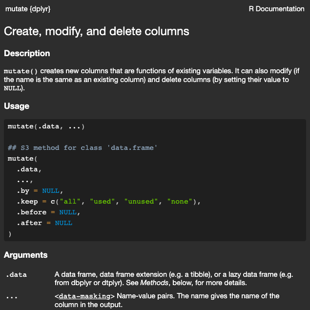
Look up the documentation of the function!

The two most common sub-types of tidy evaluation are data-masking¹ and tidy-selection².

1. Used in functions like arrange(), filter(), and summarize() that compute with variables.

2. Used in functions like select(), relocate(), and rename() that select variables.

Data Frame Function Examples

summary6 <- function(data, var) {
  data |> summarize(
    min = min({{ var }}, na.rm = TRUE),
    mean = mean({{ var }}, na.rm = TRUE),
    median = median({{ var }}, na.rm = TRUE),
    max = max({{ var }}, na.rm = TRUE),
    n = n(),
    n_miss = sum(is.na({{ var }})),
    .groups = "drop"
  )
}

diamonds |> summary6(carat)

2

The goal of this function is to compute six common summary statistics for a specified variable of a dataset.

3

Whenever you wrap summarize() in a helper function it’s good practice to set .groups = "drop" to both avoid the message and leave the data in an ungrouped state.

> # A tibble: 1 × 6
>     min  mean median   max     n n_miss
>   <dbl> <dbl>  <dbl> <dbl> <int>  <int>
> 1   0.2 0.798    0.7  5.01 53940      0

Data Frame Function Examples

count_prop <- function(df, var, sort = FALSE) {
  df |>
    count({{ var }}, sort = sort) |>
    mutate(prop = n / sum(n))
}

diamonds |> count_prop(clarity)

4

This function is a variation of count() which also calculates the proportion (Source).

> # A tibble: 8 × 3
>   clarity     n   prop
>   <ord>   <int>  <dbl>
> 1 I1        741 0.0137
> 2 SI2      9194 0.170 
> 3 SI1     13065 0.242 
> 4 VS2     12258 0.227 
> 5 VS1      8171 0.151 
> 6 VVS2     5066 0.0939
> 7 VVS1     3655 0.0678
> 8 IF       1790 0.0332

Plot Functions

What are Plot Functions?

What if you have a lot of similar plots to create? You can use a function to eliminate redundency.

The same technique can be used if you want to write a function that returns a plot since aes() is a data-masking function.

Simply use embracing within the aes() call to ggplot()!

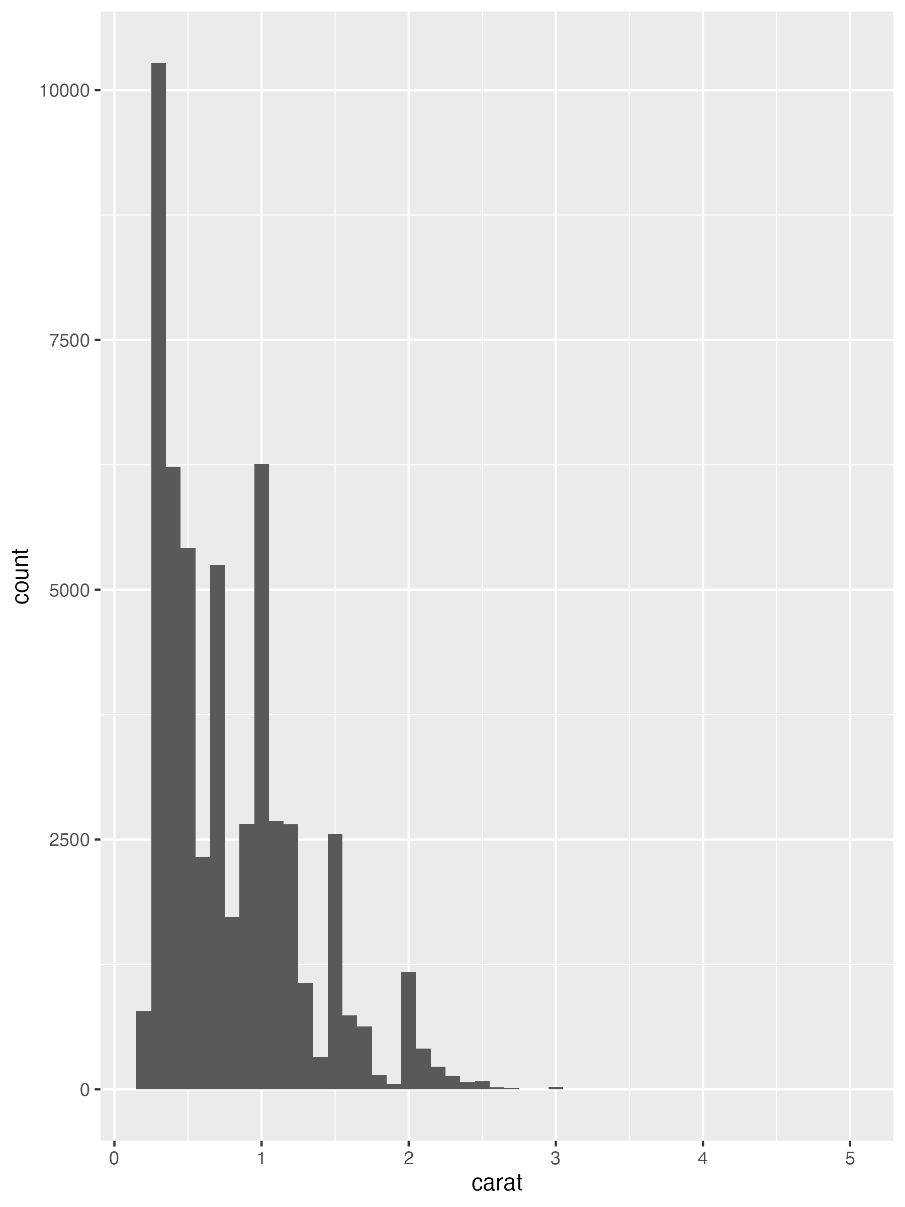
histogram <- function(df, var, binwidth = NULL) {
  df |> 
    ggplot(aes(x = {{ var }})) +
    geom_histogram(binwidth = binwidth)
}

diamonds |> histogram(carat, 0.1)

1

This is a useful function for quickly getting histograms of a specified binwidth from a dataset.

2

Note that histogram() returns a ggplot2 plot, meaning you can still add on additional components if you want. Just remember to switch from |> to +.

Data Manipulation & Plotting

You might want to create a function that has a bit of data manipulation and returns a plot.

sorted_bars <- function(df, var) {
  df |> 
    mutate({{ var }} := fct_rev(fct_infreq({{ var }})))  |>
    ggplot(aes(y = {{ var }})) + 
    geom_bar() 
}

diamonds |> sorted_bars(clarity)

3

This function creates a vertical bar chart where you automatically sort the bars in frequency order using fct_infreq().

4

:= (commonly referred to as the “walrus operator”) is used here because we are generating the variable name based on user-supplied data. R’s syntax doesn’t allow anything to the left of = except for a single, literal name. To work around this problem, we use the special operator := which tidy evaluation treats in exactly the same way as =.

Functions that Label

What if we want to add labels using our function?

For that we need to use the low-level package rlang that’s used by just about every other package in the tidyverse because it implements tidy evaluation (as well as many other useful tools).

Let’s take our histogram example from before:

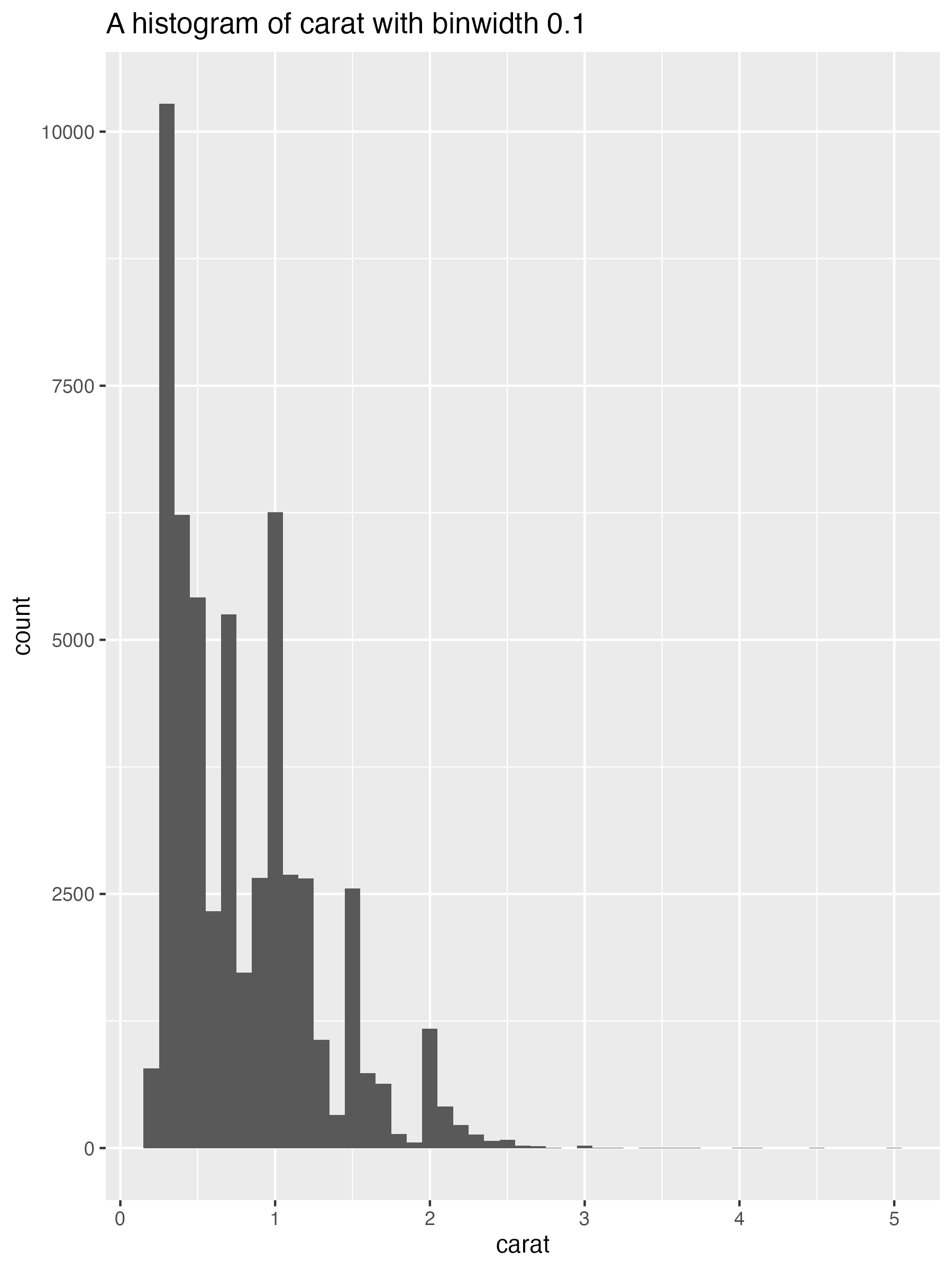
histogram <- function(df, var, binwidth) {
  label <- rlang::englue("A histogram of {{ var }} with binwidth {binwidth}")
  
  df |> 
    ggplot(aes(x = {{ var }})) + 
    geom_histogram(binwidth = binwidth) + 
    labs(title = label)
}

diamonds |> histogram(carat, 0.1)

5

rlang::englue() works similarly to str_glue(), so any value wrapped in
{ } will be inserted into the string. But it also understands { }, which automatically inserts the appropriate variable name.

Function Style Guide

Best Practices

• Make function names descriptive; again longer is better due to RStudio’s auto-complete feature.
• Generally, function names should be verbs, and arguments should be nouns.
  • Some exceptions: computation of a well-known noun (i.e. mean()), accessing a property of an object (i.e. coef())
• function() should always be followed by squiggly brackets ({}), and the contents should be indented by an additional two spaces¹.
• You should put extra spaces inside of { }. This makes it very obvious that something unusual is happening.

You can read the official tidyverse style guide for functions here.

1. This makes it easier to see the hierarchy in your code by skimming the left-hand margin.

Lab

Writing Functions

1. Practice turning the following code snippets into functions. Think about what each function does. What would you call it? How many arguments does it need?

mean(is.na(x))
mean(is.na(y))
mean(is.na(z))

x / sum(x, na.rm = TRUE)
y / sum(y, na.rm = TRUE)
z / sum(z, na.rm = TRUE)

round(x / sum(x, na.rm = TRUE) * 100, 1)
round(y / sum(y, na.rm = TRUE) * 100, 1)
round(z / sum(z, na.rm = TRUE) * 100, 1)

2. Bonus: Write a function that takes a name as an input (i.e. a character string) and returns a greeting based on the current time of day. Hint: use a time argument that defaults to lubridate::now(). That will make it easier to test your function.

Answers

1. Practice turning the following code snippets into functions. Think about what each function does. What would you call it? How many arguments does it need?

mean(is.na(x))
mean(is.na(y))
mean(is.na(z))

prop_na <- function(x){
  mean(is.na(x))
}

set.seed(50)
values <- sample(c(seq(1, 10, 1), NA), 5, replace = TRUE)
values

1

set.seed() is a function that can be used to create reproducible results when writing code that involves creating variables that take on random values.

> [1] NA  4  2  7  3

prop_na(values)

> [1] 0.2

This code calculates the proportion of NA values in a vector. I would call it prop_na() which would take a single argument, x, and return a single numeric value, between 0 and 1.

Answers

1. Practice turning the following code snippets into functions. Think about what each function does. What would you call it? How many arguments does it need?

x / sum(x, na.rm = TRUE)
y / sum(y, na.rm = TRUE)
z / sum(z, na.rm = TRUE)

sums_to_one <- function(x, na.rm = FALSE) {
  x / sum(x, na.rm = na.rm)
}

sums_to_one(values)

> [1] NA NA NA NA NA

sums_to_one(values, na.rm = TRUE)

> [1]     NA 0.2500 0.1250 0.4375 0.1875

This code standardizes a vector so that it sums to one. It takes a numeric vector and an optional specification for removing NAs. While the original code had na.rm = TRUE, it’s best to set the default to FALSE which will alert the user if NAs are present by returning NA.

Answers

1. Practice turning the following code snippets into functions. Think about what each function does. What would you call it? How many arguments does it need?

round(x / sum(x, na.rm = TRUE) * 100, 1)
round(y / sum(y, na.rm = TRUE) * 100, 1)
round(z / sum(z, na.rm = TRUE) * 100, 1)

pct_vec <- function(x, na.rm = FALSE){
  round(x / sum(x, na.rm = na.rm) * 100, 1)
}

pct_vec(values, na.rm = TRUE)

> [1]   NA 25.0 12.5 43.8 18.8

This code takes a numeric vector and finds what each value represents as a percentage of the sum of the entire vector and rounds it to the first decimal place. There is also an optional na.rm argument set to FALSE by default.

Answers

2. Bonus: Write a function that takes a name as an input (i.e. a character string) and returns a greeting based on the current time of day. Hint 1: use a time argument that defaults to lubridate::now(). That will make it easier to test your function. Hint 2: Use rlang::englue to combine your greetings with the name input.

greet <- function(name, time = now()){
  hr <- hour(time) 
  greeting <- case_when(hr < 12 & hr >= 5 ~ rlang::englue("Good morning {name}."),
                        hr < 17 & hr >= 12 ~ rlang::englue("Good afternoon {name}."),
                        hr >= 17 ~ rlang::englue("Good evening {name}."),
                        .default = rlang::englue("Why are you awake rn, {name}???"))
  return(greeting)
}

greet("Vic")

2

By default this function will take the current time to determine the specific greeting.

3

Using englue() allows you to include user-specified values with { }.

4

return() or print() or simply calling the variable greeting is necessary for the function to work as expected.

5

The last time this lecture (and therefore this code) was rendered was at 2024-05-20 12:07:04.633724

> [1] "Good afternoon Vic."

greet("Vic", time = ymd_h("2024-05-14 2am"))

> [1] "Why are you awake rn, Vic???"

Homework