- 1
- Wrapping an entire object assignment in parentheses simultaneously defines the object and shows you what it represents.
[1] 1 2Manipulating and Summarizing Data
CS&SS 508 • Lecture 4
21 October 2025
Victoria Sass
R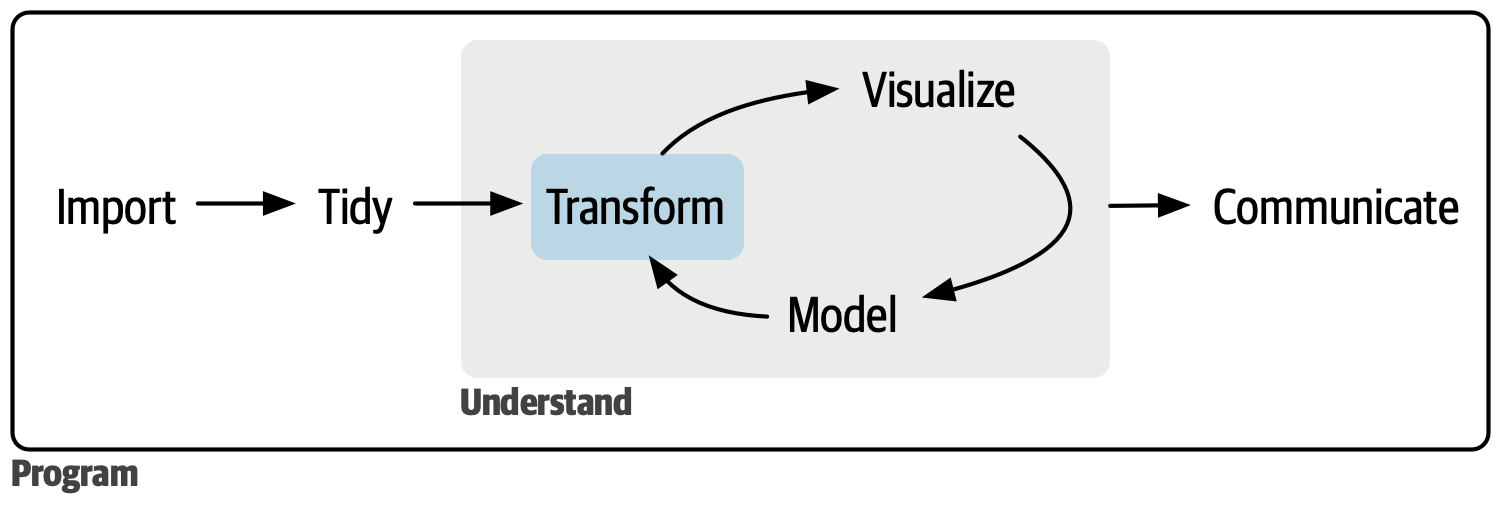
Tools like Excel or Google Sheets let you manipulate spreadsheets using functions.
Today, we’ll use R to manipulate data more transparently and reproducibly.
R?Under the hood, R stores different types of data in different ways.
4.0 is a number, and that "Vic" is not a number.So what exactly are the common data types, and how do we know what R is doing?
logical)factor)Date, POSIXct, POSIXt)integer, double)NA, NaN, Inf)character)c(FALSE, TRUE, TRUE)factor(c("red", "blue"))as_Date(c("2018-10-04"))c(1, 10*3, 4, -3.14)c(NA, NA, NA, NaN, NaN, NA)c("red", "blue", "blue")The simplest data type is a Boolean, or binary, variable: TRUE or FALSE1.
More often than not our data don’t actually have a variable with this data type, but they are definitely created and evaluated in the data manipulation and summarizing process.
Logical operators refer to base functions which allow us to test if a condition is present between two objects.
For example, we may test
Naturally, these types of expressions produce a binary outcome of T or F which enables us to transform our data in a variety of ways!
R==:!=:>, >=, <, <=:%in%:&:|:!:xor():TRUE becomes FALSE, vice versa)Be careful using == with numbers:
[1] 1 2Similarly mysterious, missing values (NA) represent the unknown. Almost anything conditional involving NAs will also be unknown:
Let’s create two objects, A and B
Comparisons:
Combinations:
B < 10 | > 20). The code won’t technically error but it won’t evaluate the way you expect it to. Read more about the confusing logic behind this here. In essence the truncated second part of this conditional statement (> 20) will evaluate to TRUE since any numeric that isn’t 0 for a logical operator is coerced to TRUE. Therefore this statement will actually always evaluate to TRUE and will return all elements of B instead of the ones that meet your specified condition.
[1] FALSE  TRUE  TRUE
[1]  TRUE FALSE  TRUE
[1] TRUE FALSE TRUEany():all():|; it’ll return TRUE if there are any TRUE’s in x&; it’ll return TRUE only if all values of x are TRUE’sif_else()
If you want to use one value when a condition is TRUE and another value when it’s FALSE.
case_when()
A very useful extension of if_else() for multiple conditions1.
.default if you want to create a “default”/catch all value.
NA and everything.
[1] "-ve" "-ve" "-ve" "0" "+ve" "+ve" "+ve" "???"dplyrToday, we’ll use tools from the dplyr package to manipulate data!
ggplot2, dplyr is part of the Tidyverse, and included in the tidyverse package.To demonstrate data transformations we’re going to use the nycflights13 dataset, which you’ll need to download and load into R
nycflights13 includes five data frames1:, some of which contain missing data (NA):
dplyr BasicsAll dplyr functions have the following in common:
Each function operates either on rows, columns, groups, or entire tables.
To save the transformations you’ve made to a data frame you’ll need to save the output to a new object.
filter()We often get big datasets, and we only want some of the entries. We can subset rows using filter().
== not = to test the logical condition.
delay_2hr is an object in our environment which contains rows corresponding to flights that experienced at least a 2 hour delay.
# A tibble: 9,723 × 19
    year month   day dep_time sched_dep_time dep_delay arr_time sched_arr_time
   <int> <int> <int>    <int>          <int>     <dbl>    <int>          <int>
 1  2013     1     1      848           1835       853     1001           1950
 2  2013     1     1      957            733       144     1056            853
 3  2013     1     1     1114            900       134     1447           1222
 4  2013     1     1     1540           1338       122     2020           1825
 5  2013     1     1     1815           1325       290     2120           1542
 6  2013     1     1     1842           1422       260     1958           1535
 7  2013     1     1     1856           1645       131     2212           2005
 8  2013     1     1     1934           1725       129     2126           1855
 9  2013     1     1     1938           1703       155     2109           1823
10  2013     1     1     1942           1705       157     2124           1830
# ℹ 9,713 more rows
# ℹ 11 more variables: arr_delay <dbl>, carrier <chr>, flight <int>,
#   tailnum <chr>, origin <chr>, dest <chr>, air_time <dbl>, distance <dbl>,
# hour <dbl>, minute <dbl>, time_hour <dttm>select()What if we want to keep every observation, but only use certain variables? Use select()!
We can select columns by name:
- before a variable name or a vector of variables to drop them from the data (i.e. select(-c(year, month, day))).
# A tibble: 336,776 × 3
    year month   day
   <int> <int> <int>
 1  2013     1     1
 2  2013     1     1
 3  2013     1     1
 4  2013     1     1
 5  2013     1     1
 6  2013     1     1
 7  2013     1     1
 8  2013     1     1
 9  2013     1     1
10  2013     1     1
# ℹ 336,766 more rowsselect()What if we want to keep every observation, but only use certain variables? Use select()!
We can select columns between variables (inclusive):
select()What if we want to keep every observation, but only use certain variables? Use select()!
We can select columns based on a condition:
select() including starts_with(), ends_with(), contains() and num_range(). Read more about these and more here.
# A tibble: 336,776 × 4
   carrier tailnum origin dest
   <chr>   <chr>   <chr>  <chr>
 1 UA      N14228  EWR    IAH
 2 UA      N24211  LGA    IAH
 3 AA      N619AA  JFK    MIA
 4 B6      N804JB  JFK    BQN
 5 DL      N668DN  LGA    ATL
 6 UA      N39463  EWR    ORD
 7 B6      N516JB  EWR    FLL
 8 EV      N829AS  LGA    IAD
 9 B6      N593JB  JFK    MCO
10 AA      N3ALAA  LGA    ORD
# ℹ 336,766 more rowsdistinct()You may want to find the unique combinations of variables in a dataset. Use distinct()
distinct() drops variables!By default, distinct() drops unused variables. If you don’t want to drop them, add the argument .keep_all = TRUE:
distinct() will find the first occurrence of a unique row in the dataset and discard the rest. Use count() if you’re looking for the number of occurrences.
# A tibble: 224 × 19
    year month   day dep_time sched_dep_time dep_delay arr_time sched_arr_time
   <int> <int> <int>    <int>          <int>     <dbl>    <int>          <int>
 1  2013     1     1      517            515         2      830            819
 2  2013     1     1      533            529         4      850            830
 3  2013     1     1      542            540         2      923            850
 4  2013     1     1      544            545        -1     1004           1022
 5  2013     1     1      554            600        -6      812            837
 6  2013     1     1      554            558        -4      740            728
 7  2013     1     1      555            600        -5      913            854
 8  2013     1     1      557            600        -3      709            723
 9  2013     1     1      557            600        -3      838            846
10  2013     1     1      558            600        -2      753            745
# ℹ 214 more rows
# ℹ 11 more variables: arr_delay <dbl>, carrier <chr>, flight <int>,
#   tailnum <chr>, origin <chr>, dest <chr>, air_time <dbl>, distance <dbl>,
# hour <dbl>, minute <dbl>, time_hour <dttm>count()sort = TRUE arranges them in descending order of number of occurrences.
# A tibble: 224 × 3
   origin dest      n
   <chr>  <chr> <int>
 1 JFK    LAX   11262
 2 LGA    ATL   10263
 3 LGA    ORD    8857
 4 JFK    SFO    8204
 5 LGA    CLT    6168
 6 EWR    ORD    6100
 7 JFK    BOS    5898
 8 LGA    MIA    5781
 9 JFK    MCO    5464
10 EWR    BOS    5327
# ℹ 214 more rowsarrange()Sometimes it’s useful to sort rows in your data, in ascending (low to high) or descending (high to low) order. We do that with arrange().
# A tibble: 336,776 × 19
    year month   day dep_time sched_dep_time dep_delay arr_time sched_arr_time
   <int> <int> <int>    <int>          <int>     <dbl>    <int>          <int>
 1  2013     1     1      517            515         2      830            819
 2  2013     1     1      533            529         4      850            830
 3  2013     1     1      542            540         2      923            850
 4  2013     1     1      544            545        -1     1004           1022
 5  2013     1     1      554            600        -6      812            837
 6  2013     1     1      554            558        -4      740            728
 7  2013     1     1      555            600        -5      913            854
 8  2013     1     1      557            600        -3      709            723
 9  2013     1     1      557            600        -3      838            846
10  2013     1     1      558            600        -2      753            745
# ℹ 336,766 more rows
# ℹ 11 more variables: arr_delay <dbl>, carrier <chr>, flight <int>,
#   tailnum <chr>, origin <chr>, dest <chr>, air_time <dbl>, distance <dbl>,
# hour <dbl>, minute <dbl>, time_hour <dttm>arrange()To sort in descending order, using desc() within arrange()
# A tibble: 336,776 × 19
    year month   day dep_time sched_dep_time dep_delay arr_time sched_arr_time
   <int> <int> <int>    <int>          <int>     <dbl>    <int>          <int>
 1  2013     1     9      641            900      1301     1242           1530
 2  2013     6    15     1432           1935      1137     1607           2120
 3  2013     1    10     1121           1635      1126     1239           1810
 4  2013     9    20     1139           1845      1014     1457           2210
 5  2013     7    22      845           1600      1005     1044           1815
 6  2013     4    10     1100           1900       960     1342           2211
 7  2013     3    17     2321            810       911      135           1020
 8  2013     6    27      959           1900       899     1236           2226
 9  2013     7    22     2257            759       898      121           1026
10  2013    12     5      756           1700       896     1058           2020
# ℹ 336,766 more rows
# ℹ 11 more variables: arr_delay <dbl>, carrier <chr>, flight <int>,
#   tailnum <chr>, origin <chr>, dest <chr>, air_time <dbl>, distance <dbl>,
# hour <dbl>, minute <dbl>, time_hour <dttm>rename()You may receive data with unintuitive variable names. Change them using rename().
rename(new_name = old_name) is the format. Reminder to use janitor::clean_names() if you want to automate this process for a lot of variables.
# A tibble: 336,776 × 19
    year month   day dep_time sched_dep_time dep_delay arr_time sched_arr_time
   <int> <int> <int>    <int>          <int>     <dbl>    <int>          <int>
 1  2013     1     1      517            515         2      830            819
 2  2013     1     1      533            529         4      850            830
 3  2013     1     1      542            540         2      923            850
 4  2013     1     1      544            545        -1     1004           1022
 5  2013     1     1      554            600        -6      812            837
 6  2013     1     1      554            558        -4      740            728
 7  2013     1     1      555            600        -5      913            854
 8  2013     1     1      557            600        -3      709            723
 9  2013     1     1      557            600        -3      838            846
10  2013     1     1      558            600        -2      753            745
# ℹ 336,766 more rows
# ℹ 11 more variables: arr_delay <dbl>, carrier <chr>, flight <int>,
#   tail_num <chr>, origin <chr>, dest <chr>, air_time <dbl>, distance <dbl>,
#   hour <dbl>, minute <dbl>, time_hour <dttm>
Variable Syntax
I recommend against using spaces in a name! It makes things really hard sometimes!!
mutate()You can add new columns to a data frame using mutate().
mutate() adds new columns on the right hand side of your dataset, which makes it difficult to see if anything happened. You can use the .before argument to specify which numeric index (or variable name) to move the newly created variable to. .after is an alternative argument for this.
# A tibble: 336,776 × 21
    gain speed  year month   day dep_time sched_dep_time dep_delay arr_time
   <dbl> <dbl> <int> <int> <int>    <int>          <int>     <dbl>    <int>
 1    -9  370.  2013     1     1      517            515         2      830
 2   -16  374.  2013     1     1      533            529         4      850
 3   -31  408.  2013     1     1      542            540         2      923
 4    17  517.  2013     1     1      544            545        -1     1004
 5    19  394.  2013     1     1      554            600        -6      812
 6   -16  288.  2013     1     1      554            558        -4      740
 7   -24  404.  2013     1     1      555            600        -5      913
 8    11  259.  2013     1     1      557            600        -3      709
 9     5  405.  2013     1     1      557            600        -3      838
10   -10  319.  2013     1     1      558            600        -2      753
# ℹ 336,766 more rows
# ℹ 12 more variables: sched_arr_time <int>, arr_delay <dbl>, carrier <chr>,
#   flight <int>, tailnum <chr>, origin <chr>, dest <chr>, air_time <dbl>,
# distance <dbl>, hour <dbl>, minute <dbl>, time_hour <dttm>mutate()You can specify which columns to keep with the .keep argument:
flights |>
mutate(
gain = dep_delay - arr_delay,
hours = air_time / 60,
gain_per_hour = gain / hours,
.keep = "used"
)"used" retains only the variables used to create the new variables, which is useful for checking your work. Other options include: "all" (default, returns all columns), "unused" (columns not used to create new columns) and "none" (only grouping variables and columns created by mutate are retained).
# A tibble: 336,776 × 6
   dep_delay arr_delay air_time  gain hours gain_per_hour
       <dbl>     <dbl>    <dbl> <dbl> <dbl>         <dbl>
 1         2        11      227    -9 3.78          -2.38
 2         4        20      227   -16 3.78          -4.23
 3         2        33      160   -31 2.67         -11.6
 4        -1       -18      183    17 3.05           5.57
 5        -6       -25      116    19 1.93           9.83
 6        -4        12      150   -16 2.5           -6.4
 7        -5        19      158   -24 2.63          -9.11
 8        -3       -14       53    11 0.883         12.5
 9        -3        -8      140     5 2.33           2.14
10        -2         8      138   -10 2.3           -4.35
# ℹ 336,766 more rowsrelocate()You might want to collect related variables together or move important variables to the front. Use relocate()!
relocate() moves variables to the front but you can also specify where to put them using the .before and .after arguments, just like in mutate().
# A tibble: 336,776 × 19
   time_hour           air_time  year month   day dep_time sched_dep_time
   <dttm>                 <dbl> <int> <int> <int>    <int>          <int>
 1 2013-01-01 05:00:00      227  2013     1     1      517            515
 2 2013-01-01 05:00:00      227  2013     1     1      533            529
 3 2013-01-01 05:00:00      160  2013     1     1      542            540
 4 2013-01-01 05:00:00      183  2013     1     1      544            545
 5 2013-01-01 06:00:00      116  2013     1     1      554            600
 6 2013-01-01 05:00:00      150  2013     1     1      554            558
 7 2013-01-01 06:00:00      158  2013     1     1      555            600
 8 2013-01-01 06:00:00       53  2013     1     1      557            600
 9 2013-01-01 06:00:00      140  2013     1     1      557            600
10 2013-01-01 06:00:00      138  2013     1     1      558            600
# ℹ 336,766 more rows
# ℹ 12 more variables: dep_delay <dbl>, arr_time <int>, sched_arr_time <int>,
#   arr_delay <dbl>, carrier <chr>, flight <int>, tailnum <chr>, origin <chr>,
# dest <chr>, distance <dbl>, hour <dbl>, minute <dbl>group_by()If you want to analyze your data by specific groupings, use group_by():
group_by() doesn’t change the data but you’ll notice that the output indicates that it is “grouped by” month (Groups: month [12]). This means subsequent operations will now work “by month”.
# A tibble: 336,776 × 19
# Groups:   month [12]
    year month   day dep_time sched_dep_time dep_delay arr_time sched_arr_time
   <int> <int> <int>    <int>          <int>     <dbl>    <int>          <int>
 1  2013     1     1      517            515         2      830            819
 2  2013     1     1      533            529         4      850            830
 3  2013     1     1      542            540         2      923            850
 4  2013     1     1      544            545        -1     1004           1022
 5  2013     1     1      554            600        -6      812            837
 6  2013     1     1      554            558        -4      740            728
 7  2013     1     1      555            600        -5      913            854
 8  2013     1     1      557            600        -3      709            723
 9  2013     1     1      557            600        -3      838            846
10  2013     1     1      558            600        -2      753            745
# ℹ 336,766 more rows
# ℹ 11 more variables: arr_delay <dbl>, carrier <chr>, flight <int>,
#   tailnum <chr>, origin <chr>, dest <chr>, air_time <dbl>, distance <dbl>,
# hour <dbl>, minute <dbl>, time_hour <dttm>summarize()summarize() calculates summaries of variables in your data:
You can use any function inside summarize() that aggregates multiple values into a single value (like sd(), mean(), or max()).
summarize() ExampleLet’s see what this looks like in our flights dataset:
summarize() ExampleLet’s see what this looks like in our flights dataset:
What if we want to summarize data by our groups? Use group_by() and summarize()
Because we did group_by() with month, then used summarize(), we get one row per value of month!
You can create any number of summaries in a single call to summarize().
n() returns the number of rows in each group.
# A tibble: 12 × 3
   month delay     n
   <int> <dbl> <int>
 1     1 10.0  27004
 2     2 10.8  24951
 3     3 13.2  28834
 4     4 13.9  28330
 5     5 13.0  28796
 6     6 20.8  28243
 7     7 21.7  29425
 8     8 12.6  29327
 9     9  6.72 27574
10    10  6.24 28889
11    11  5.44 27268
12 12 16.6 28135# A tibble: 336,776 × 19
# Groups: year, month, day [365]
year month day dep_time sched_dep_time dep_delay arr_time sched_arr_time
<int> <int> <int> <int> <int> <dbl> <int> <int>
1 2013 1 1 517 515 2 830 819
2 2013 1 1 533 529 4 850 830
3 2013 1 1 542 540 2 923 850
4 2013 1 1 544 545 -1 1004 1022
5 2013 1 1 554 600 -6 812 837
6 2013 1 1 554 558 -4 740 728
7 2013 1 1 555 600 -5 913 854
8 2013 1 1 557 600 -3 709 723
9 2013 1 1 557 600 -3 838 846
10 2013 1 1 558 600 -2 753 745
# ℹ 336,766 more rows
# ℹ 11 more variables: arr_delay <dbl>, carrier <chr>, flight <int>,
# tailnum <chr>, origin <chr>, dest <chr>, air_time <dbl>, distance <dbl>,
# hour <dbl>, minute <dbl>, time_hour <dttm>Summary & Grouping Behavior
When you summarize a tibble grouped by more than one variable, each summary peels off the last group. You can change the default behavior by setting the .groups argument to a different value, e.g., "drop" to drop all grouping or "keep" to preserve the same groups. The default is "drop_last" if all groups have 1 row and keep otherwise (it’s recommended to use reframe() if this is the case, which is a more general version of summarize() that allows for an arbitrary number of rows per group and drops all grouping variables after execution).
ungroup()# A tibble: 336,776 × 19
year month day dep_time sched_dep_time dep_delay arr_time sched_arr_time
<int> <int> <int> <int> <int> <dbl> <int> <int>
1 2013 1 1 517 515 2 830 819
2 2013 1 1 533 529 4 850 830
3 2013 1 1 542 540 2 923 850
4 2013 1 1 544 545 -1 1004 1022
5 2013 1 1 554 600 -6 812 837
6 2013 1 1 554 558 -4 740 728
7 2013 1 1 555 600 -5 913 854
8 2013 1 1 557 600 -3 709 723
9 2013 1 1 557 600 -3 838 846
10 2013 1 1 558 600 -2 753 745
# ℹ 336,766 more rows
# ℹ 11 more variables: arr_delay <dbl>, carrier <chr>, flight <int>,
# tailnum <chr>, origin <chr>, dest <chr>, air_time <dbl>, distance <dbl>,
# hour <dbl>, minute <dbl>, time_hour <dttm>.by.by works with all verbs and has the advantage that you don’t need to use the .groups argument to suppress the grouping message or ungroup() when you’re done.
# A tibble: 12 × 3
   month delay     n
   <int> <dbl> <int>
 1     1 10.0  27004
 2    10  6.24 28889
 3    11  5.44 27268
 4    12 16.6  28135
 5     2 10.8  24951
 6     3 13.2  28834
 7     4 13.9  28330
 8     5 13.0  28796
 9     6 20.8  28243
10     7 21.7  29425
11     8 12.6  29327
12 9 6.72 27574slice_*There are five handy functions that allow you extract specific rows within each group:
df |> slice_head(n = 1) takes the first row from each group.df |> slice_tail(n = 1) takes the last row in each group.df |> slice_min(x, n = 1) takes the row with the smallest value of column x.df |> slice_max(x, n = 1) takes the row with the largest value of column x.df |> slice_sample(n = 1) takes one random row.Let’s find the flights that are most delayed upon arrival at each destination.
slice_*n to select more than one row, or instead of n, you can use prop to select a proportion (between 0 and 1) of the rows in each group.
# A tibble: 108 × 19
# Groups:   dest [105]
   dest  arr_delay  year month   day dep_time sched_dep_time dep_delay arr_time
   <chr>     <dbl> <int> <int> <int>    <int>          <int>     <dbl>    <int>
 1 ABQ         153  2013     7    22     2145           2007        98      132
 2 ACK         221  2013     7    23     1139            800       219     1250
 3 ALB         328  2013     1    25      123           2000       323      229
 4 ANC          39  2013     8    17     1740           1625        75     2042
 5 ATL         895  2013     7    22     2257            759       898      121
 6 AUS         349  2013     7    10     2056           1505       351     2347
 7 AVL         228  2013     8    13     1156            832       204     1417
 8 BDL         266  2013     2    21     1728           1316       252     1839
 9 BGR         238  2013    12     1     1504           1056       248     1628
10 BHM         291  2013     4    10       25           1900       325      136
# ℹ 98 more rows
# ℹ 10 more variables: sched_arr_time <int>, carrier <chr>, flight <int>,
#   tailnum <chr>, origin <chr>, air_time <dbl>, distance <dbl>, hour <dbl>,
# minute <dbl>, time_hour <dttm>gapminder1
year (ascending order) and population (descending order) and save that over (i.e. overwrite) the object created for answer 1. Print the first 6 rows.ggplot, create a line plot showing life expectancy over time by country. Make the plot visually appealing!Question 1:
subset_gapminder <- gapminder |>
filter(country %in% c("China","India","United States"), year > 1980 ) |>
select(country, year, pop, lifeExp)
subset_gapminderfilter() by separating them with commas
# A tibble: 18 × 4
   country        year        pop lifeExp
   <fct>         <int>      <int>   <dbl>
 1 China          1982 1000281000    65.5
 2 China          1987 1084035000    67.3
 3 China          1992 1164970000    68.7
 4 China          1997 1230075000    70.4
 5 China          2002 1280400000    72.0
 6 China          2007 1318683096    73.0
 7 India          1982  708000000    56.6
 8 India          1987  788000000    58.6
 9 India          1992  872000000    60.2
10 India          1997  959000000    61.8
11 India          2002 1034172547    62.9
12 India          2007 1110396331    64.7
13 United States  1982  232187835    74.6
14 United States  1987  242803533    75.0
15 United States  1992  256894189    76.1
16 United States  1997  272911760    76.8
17 United States  2002  287675526    77.3
18 United States 2007 301139947 78.2Question 2:
[1] 18 4Rows: 18
Columns: 4
$ country <fct> "China", "China", "China", "China", "China", "China", "India",…
$ year <int> 1982, 1987, 1992, 1997, 2002, 2007, 1982, 1987, 1992, 1997, 20…
$ pop <int> 1000281000, 1084035000, 1164970000, 1230075000, 1280400000, 13…
$ lifeExp <dbl> 65.525, 67.274, 68.690, 70.426, 72.028, 72.961, 56.596, 58.553…[1] 18 4Question 3:
arrange() is to sort in ascending order
Question 4:
# A tibble: 18 × 5
   country        year        pop lifeExp pop_billions
   <fct>         <int>      <int>   <dbl>        <dbl>
 1 China          1982 1000281000    65.5        1.00
 2 India          1982  708000000    56.6        0.708
 3 United States  1982  232187835    74.6        0.232
 4 China          1987 1084035000    67.3        1.08
 5 India          1987  788000000    58.6        0.788
 6 United States  1987  242803533    75.0        0.243
 7 China          1992 1164970000    68.7        1.16
 8 India          1992  872000000    60.2        0.872
 9 United States  1992  256894189    76.1        0.257
10 China          1997 1230075000    70.4        1.23
11 India          1997  959000000    61.8        0.959
12 United States  1997  272911760    76.8        0.273
13 China          2002 1280400000    72.0        1.28
14 India          2002 1034172547    62.9        1.03
15 United States  2002  287675526    77.3        0.288
16 China          2007 1318683096    73.0        1.32
17 India          2007 1110396331    64.7        1.11
18 United States 2007 301139947 78.2 0.301Question 5:
ungroup() is called). Learn more about this new feature here)
# A tibble: 6 × 2
   year TotalPop_Billions
  <int>             <dbl>
1  1982              1.94
2  1987              2.11
3  1992              2.29
4  1997              2.46
5  2002              2.60
6 2007 2.73Question 6:
library(ggplot2)
library(ggthemes)
library(geomtextpath)
ggplot(subset_gapminder,
aes(year, lifeExp, color = country)) +
geom_point() +
geom_textpath(aes(label = country),
show.legend = FALSE) +
labs(title = "Life Expectancy (1982-2007)","China, India, and United States",
x = "Year",
y = "Life Expectancy (years)") +
scale_x_continuous(breaks = c(1982, 1987, 1992, 1997, 2002, 2007)) +
ylim(c(50, 80)) +
theme_tufte(base_size = 20)year to the x-axis, lifeExp to the y-axis, and country to color
geom_textpath() from the geomtextpath package to make nice labelled lines (specify mapping of country to the label)
ggthemes package and increase text size throughout plot
In practice, we often collect data from different sources. To analyze the data, we usually must first combine (merge) them.
For example, imagine you would like to study county-level patterns with respect to age and grocery spending. However, you can only find,
Merge the data!!
To do this we’ll be using the various join functions from the dplyr package.
We need to think about the following when we want to merge data frames A and B:
Keys are the way that two datasets are connected to one another. The two types of keys are:
Let’s look at our data to gain a better sense of what this all means.
airlines records two pieces of data about each airline: its carrier code and its full name. You can identify an airline with its two letter carrier code, making carrier the primary key.
glimpse on any dataset to see a transposed version of the data, making it possible to see all available column names, types, and a preview of as many values will fit on your current screen.
Rows: 16
Columns: 2
$ carrier <chr> "9E", "AA", "AS", "B6", "DL", "EV", "F9", "FL", "HA", "MQ", "O…
$ name    <chr> "Endeavor Air Inc.", "American Airlines Inc.", "Alaska Airline…
airports records data about each airport. You can identify each airport by its three letter airport code, making faa the primary key.
Rows: 1,458
Columns: 8
$ faa   <chr> "04G", "06A", "06C", "06N", "09J", "0A9", "0G6", "0G7", "0P2", "…
$ name  <chr> "Lansdowne Airport", "Moton Field Municipal Airport", "Schaumbur…
$ lat   <dbl> 41.13047, 32.46057, 41.98934, 41.43191, 31.07447, 36.37122, 41.4…
$ lon   <dbl> -80.61958, -85.68003, -88.10124, -74.39156, -81.42778, -82.17342…
$ alt   <dbl> 1044, 264, 801, 523, 11, 1593, 730, 492, 1000, 108, 409, 875, 10…
$ tz    <dbl> -5, -6, -6, -5, -5, -5, -5, -5, -5, -8, -5, -6, -5, -5, -5, -5, …
$ dst   <chr> "A", "A", "A", "A", "A", "A", "A", "A", "U", "A", "A", "U", "A",…
$ tzone <chr> "America/New_York", "America/Chicago", "America/Chicago", "Ameri…
planes records data about each plane. You can identify a plane by its tail number, making tailnum the primary key.
Rows: 3,322
Columns: 9
$ tailnum      <chr> "N10156", "N102UW", "N103US", "N104UW", "N10575", "N105UW…
$ year         <int> 2004, 1998, 1999, 1999, 2002, 1999, 1999, 1999, 1999, 199…
$ type         <chr> "Fixed wing multi engine", "Fixed wing multi engine", "Fi…
$ manufacturer <chr> "EMBRAER", "AIRBUS INDUSTRIE", "AIRBUS INDUSTRIE", "AIRBU…
$ model        <chr> "EMB-145XR", "A320-214", "A320-214", "A320-214", "EMB-145…
$ engines      <int> 2, 2, 2, 2, 2, 2, 2, 2, 2, 2, 2, 2, 2, 2, 2, 2, 2, 2, 2, …
$ seats        <int> 55, 182, 182, 182, 55, 182, 182, 182, 182, 182, 55, 55, 5…
$ speed        <int> NA, NA, NA, NA, NA, NA, NA, NA, NA, NA, NA, NA, NA, NA, N…
$ engine       <chr> "Turbo-fan", "Turbo-fan", "Turbo-fan", "Turbo-fan", "Turb…
weather records data about the weather at the origin airports. You can identify each observation by the combination of location and time, making origin and time_hour the compound primary key.
Rows: 26,115
Columns: 15
$ origin     <chr> "EWR", "EWR", "EWR", "EWR", "EWR", "EWR", "EWR", "EWR", "EW…
$ year       <int> 2013, 2013, 2013, 2013, 2013, 2013, 2013, 2013, 2013, 2013,…
$ month      <int> 1, 1, 1, 1, 1, 1, 1, 1, 1, 1, 1, 1, 1, 1, 1, 1, 1, 1, 1, 1,…
$ day        <int> 1, 1, 1, 1, 1, 1, 1, 1, 1, 1, 1, 1, 1, 1, 1, 1, 1, 1, 1, 1,…
$ hour       <int> 1, 2, 3, 4, 5, 6, 7, 8, 9, 10, 11, 13, 14, 15, 16, 17, 18, …
$ temp       <dbl> 39.02, 39.02, 39.02, 39.92, 39.02, 37.94, 39.02, 39.92, 39.…
$ dewp       <dbl> 26.06, 26.96, 28.04, 28.04, 28.04, 28.04, 28.04, 28.04, 28.…
$ humid      <dbl> 59.37, 61.63, 64.43, 62.21, 64.43, 67.21, 64.43, 62.21, 62.…
$ wind_dir   <dbl> 270, 250, 240, 250, 260, 240, 240, 250, 260, 260, 260, 330,…
$ wind_speed <dbl> 10.35702, 8.05546, 11.50780, 12.65858, 12.65858, 11.50780, …
$ wind_gust  <dbl> NA, NA, NA, NA, NA, NA, NA, NA, NA, NA, NA, NA, NA, NA, 20.…
$ precip     <dbl> 0, 0, 0, 0, 0, 0, 0, 0, 0, 0, 0, 0, 0, 0, 0, 0, 0, 0, 0, 0,…
$ pressure   <dbl> 1012.0, 1012.3, 1012.5, 1012.2, 1011.9, 1012.4, 1012.2, 101…
$ visib      <dbl> 10, 10, 10, 10, 10, 10, 10, 10, 10, 10, 10, 10, 10, 10, 10,…
$ time_hour  <dttm> 2013-01-01 01:00:00, 2013-01-01 02:00:00, 2013-01-01 03:00…
flights has three variables (time_hour, flight, carrier) that uniquely identify an observation. More significantly, however, it contains foreign keys that correspond to the primary keys of the other datasets.
Rows: 336,776
Columns: 19
$ year           <int> 2013, 2013, 2013, 2013, 2013, 2013, 2013, 2013, 2013, 2…
$ month          <int> 1, 1, 1, 1, 1, 1, 1, 1, 1, 1, 1, 1, 1, 1, 1, 1, 1, 1, 1…
$ day            <int> 1, 1, 1, 1, 1, 1, 1, 1, 1, 1, 1, 1, 1, 1, 1, 1, 1, 1, 1…
$ dep_time       <int> 517, 533, 542, 544, 554, 554, 555, 557, 557, 558, 558, …
$ sched_dep_time <int> 515, 529, 540, 545, 600, 558, 600, 600, 600, 600, 600, …
$ dep_delay      <dbl> 2, 4, 2, -1, -6, -4, -5, -3, -3, -2, -2, -2, -2, -2, -1…
$ arr_time       <int> 830, 850, 923, 1004, 812, 740, 913, 709, 838, 753, 849,…
$ sched_arr_time <int> 819, 830, 850, 1022, 837, 728, 854, 723, 846, 745, 851,…
$ arr_delay      <dbl> 11, 20, 33, -18, -25, 12, 19, -14, -8, 8, -2, -3, 7, -1…
$ carrier        <chr> "UA", "UA", "AA", "B6", "DL", "UA", "B6", "EV", "B6", "…
$ flight         <int> 1545, 1714, 1141, 725, 461, 1696, 507, 5708, 79, 301, 4…
$ tailnum        <chr> "N14228", "N24211", "N619AA", "N804JB", "N668DN", "N394…
$ origin         <chr> "EWR", "LGA", "JFK", "JFK", "LGA", "EWR", "EWR", "LGA",…
$ dest           <chr> "IAH", "IAH", "MIA", "BQN", "ATL", "ORD", "FLL", "IAD",…
$ air_time       <dbl> 227, 227, 160, 183, 116, 150, 158, 53, 140, 138, 149, 1…
$ distance       <dbl> 1400, 1416, 1089, 1576, 762, 719, 1065, 229, 944, 733, …
$ hour           <dbl> 5, 5, 5, 5, 6, 5, 6, 6, 6, 6, 6, 6, 6, 6, 6, 5, 6, 6, 6…
$ minute         <dbl> 15, 29, 40, 45, 0, 58, 0, 0, 0, 0, 0, 0, 0, 0, 0, 59, 0…
$ time_hour <dttm> 2013-01-01 05:00:00, 2013-01-01 05:00:00, 2013-01-01 0…These are variables in a dataset that refer to a primary key in another dataset. Note: pinkish shading indicates the primary key for that particular dataset.
flights$origin –> airports$faaflights$dest –> airports$faaflights$origin-flights$time_hour –> weather$origin-weather$time_hour.flights$tailnum –> planes$tailnumflights$carrier –> airlines$carrierA nice feature of these data are that the primary and foreign keys have the same name and almost every variable name used across multiple tables has the same meaning.1 This isn’t always the case!2
It is good practice to make sure your primary keys actually uniquely identify an observation and that they don’t have any missing values.
# A tibble: 0 × 2
# ℹ 2 variables: tailnum <chr>, n <int>Sometimes you’ll want to create an index of your observations to serve as a surrogate key because the compound primary key is not particularly easy to reference.
For example, our flights dataset has three variables that uniquely identify each observation: time_hour, carrier, flight.
row_number() simply specifies the row number of the data frame.
# A tibble: 336,776 × 20
      id  year month   day dep_time sched_dep_time dep_delay arr_time
   <int> <int> <int> <int>    <int>          <int>     <dbl>    <int>
 1     1  2013     1     1      517            515         2      830
 2     2  2013     1     1      533            529         4      850
 3     3  2013     1     1      542            540         2      923
 4     4  2013     1     1      544            545        -1     1004
 5     5  2013     1     1      554            600        -6      812
 6     6  2013     1     1      554            558        -4      740
 7     7  2013     1     1      555            600        -5      913
 8     8  2013     1     1      557            600        -3      709
 9     9  2013     1     1      557            600        -3      838
10    10  2013     1     1      558            600        -2      753
# ℹ 336,766 more rows
# ℹ 12 more variables: sched_arr_time <int>, arr_delay <dbl>, carrier <chr>,
#   flight <int>, tailnum <chr>, origin <chr>, dest <chr>, air_time <dbl>,
# distance <dbl>, hour <dbl>, minute <dbl>, time_hour <dttm>All join functions have the same basic interface: they take a pair of data frames and return one data frame.
The order of the rows and columns is primarily going to be determined by the first data frame.
dplyr has two types of joins: mutating and filtering.
Add new variables to one data frame from matching observations from another data frame.
left_join()right_join()inner_join()full_join()Filter observations from one data frame based on whether or not they match an observation in another data frame.
semi_join()anti-join()Mutating Joins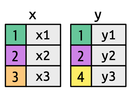
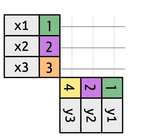
left_join()The most common type of join Appends columns from y to x by the rows in x
(NA added if there is nothing from y) Natural join: when all variables that appear in both datasets are used as the join key.
If the join_by() argument is not specified, left_join() will automatically join by all columns that have names and values in common.
left_join in nycflights13With only the pertinent variables from the flights dataset, we can see how a left_join works with the airlines dataset.
Joining with `by = join_by(carrier)`# A tibble: 336,776 × 7
year time_hour origin dest tailnum carrier name
<int> <dttm> <chr> <chr> <chr> <chr> <chr>
1 2013 2013-01-01 05:00:00 EWR IAH N14228 UA United Air Lines Inc.
2 2013 2013-01-01 05:00:00 LGA IAH N24211 UA United Air Lines Inc.
3 2013 2013-01-01 05:00:00 JFK MIA N619AA AA American Airlines Inc.
4 2013 2013-01-01 05:00:00 JFK BQN N804JB B6 JetBlue Airways
5 2013 2013-01-01 06:00:00 LGA ATL N668DN DL Delta Air Lines Inc.
6 2013 2013-01-01 05:00:00 EWR ORD N39463 UA United Air Lines Inc.
7 2013 2013-01-01 06:00:00 EWR FLL N516JB B6 JetBlue Airways
8 2013 2013-01-01 06:00:00 LGA IAD N829AS EV ExpressJet Airlines I…
9 2013 2013-01-01 06:00:00 JFK MCO N593JB B6 JetBlue Airways
10 2013 2013-01-01 06:00:00 LGA ORD N3ALAA AA American Airlines Inc.
# ℹ 336,766 more rowsplanes dataset has variables tailnum, year, type, manufacturer, model, engines, seats, speed, and engine
Joining with `by = join_by(year, tailnum)`# A tibble: 336,776 × 13
year time_hour origin dest tailnum carrier type manufacturer
<int> <dttm> <chr> <chr> <chr> <chr> <chr> <chr>
1 2013 2013-01-01 05:00:00 EWR IAH N14228 UA <NA> <NA>
2 2013 2013-01-01 05:00:00 LGA IAH N24211 UA <NA> <NA>
3 2013 2013-01-01 05:00:00 JFK MIA N619AA AA <NA> <NA>
4 2013 2013-01-01 05:00:00 JFK BQN N804JB B6 <NA> <NA>
5 2013 2013-01-01 06:00:00 LGA ATL N668DN DL <NA> <NA>
6 2013 2013-01-01 05:00:00 EWR ORD N39463 UA <NA> <NA>
7 2013 2013-01-01 06:00:00 EWR FLL N516JB B6 <NA> <NA>
8 2013 2013-01-01 06:00:00 LGA IAD N829AS EV <NA> <NA>
9 2013 2013-01-01 06:00:00 JFK MCO N593JB B6 <NA> <NA>
10 2013 2013-01-01 06:00:00 LGA ORD N3ALAA AA <NA> <NA>
# ℹ 336,766 more rows
# ℹ 5 more variables: model <chr>, engines <int>, seats <int>, speed <int>,
# engine <chr>
When we try to do this, however, we get a bunch of NAs. Why?
join_by(tailnum) is short for join_by(tailnum == tailnum) making these types of basic joins equi joins.
# A tibble: 336,776 × 14
   year.x time_hour           origin dest  tailnum carrier year.y type
    <int> <dttm>              <chr>  <chr> <chr>   <chr>    <int> <chr>
 1   2013 2013-01-01 05:00:00 EWR    IAH   N14228  UA        1999 Fixed wing mu…
 2   2013 2013-01-01 05:00:00 LGA    IAH   N24211  UA        1998 Fixed wing mu…
 3   2013 2013-01-01 05:00:00 JFK    MIA   N619AA  AA        1990 Fixed wing mu…
 4   2013 2013-01-01 05:00:00 JFK    BQN   N804JB  B6        2012 Fixed wing mu…
 5   2013 2013-01-01 06:00:00 LGA    ATL   N668DN  DL        1991 Fixed wing mu…
 6   2013 2013-01-01 05:00:00 EWR    ORD   N39463  UA        2012 Fixed wing mu…
 7   2013 2013-01-01 06:00:00 EWR    FLL   N516JB  B6        2000 Fixed wing mu…
 8   2013 2013-01-01 06:00:00 LGA    IAD   N829AS  EV        1998 Fixed wing mu…
 9   2013 2013-01-01 06:00:00 JFK    MCO   N593JB  B6        2004 Fixed wing mu…
10   2013 2013-01-01 06:00:00 LGA    ORD   N3ALAA  AA          NA <NA>
# ℹ 336,766 more rows
# ℹ 6 more variables: manufacturer <chr>, model <chr>, engines <int>,
# seats <int>, speed <int>, engine <chr>If you have keys that have the same meaning (values) but are named different things in their respective datasets you’d also specify that with join_by()
by = c("dest" = "faa") was the former syntax for this and you still might see that in older code. You can specify multiple join_bys by simply separating the conditional statements with , (i.e. join_by(x == y, a == b)).
# A tibble: 336,776 × 13
    year time_hour           origin dest  tailnum carrier name         lat   lon
   <int> <dttm>              <chr>  <chr> <chr>   <chr>   <chr>      <dbl> <dbl>
 1  2013 2013-01-01 05:00:00 EWR    IAH   N14228  UA      George Bu…  30.0 -95.3
 2  2013 2013-01-01 05:00:00 LGA    IAH   N24211  UA      George Bu…  30.0 -95.3
 3  2013 2013-01-01 05:00:00 JFK    MIA   N619AA  AA      Miami Intl  25.8 -80.3
 4  2013 2013-01-01 05:00:00 JFK    BQN   N804JB  B6      <NA>        NA    NA
 5  2013 2013-01-01 06:00:00 LGA    ATL   N668DN  DL      Hartsfiel…  33.6 -84.4
 6  2013 2013-01-01 05:00:00 EWR    ORD   N39463  UA      Chicago O…  42.0 -87.9
 7  2013 2013-01-01 06:00:00 EWR    FLL   N516JB  B6      Fort Laud…  26.1 -80.2
 8  2013 2013-01-01 06:00:00 LGA    IAD   N829AS  EV      Washingto…  38.9 -77.5
 9  2013 2013-01-01 06:00:00 JFK    MCO   N593JB  B6      Orlando I…  28.4 -81.3
10  2013 2013-01-01 06:00:00 LGA    ORD   N3ALAA  AA      Chicago O…  42.0 -87.9
# ℹ 336,766 more rows
# ℹ 4 more variables: alt <dbl>, tz <dbl>, dst <chr>, tzone <chr>You can request dplyr to keep both keys with keep = TRUE argument.
# A tibble: 336,776 × 14
    year time_hour           origin dest  tailnum carrier faa   name         lat
   <int> <dttm>              <chr>  <chr> <chr>   <chr>   <chr> <chr>      <dbl>
 1  2013 2013-01-01 05:00:00 EWR    IAH   N14228  UA      IAH   George Bu…  30.0
 2  2013 2013-01-01 05:00:00 LGA    IAH   N24211  UA      IAH   George Bu…  30.0
 3  2013 2013-01-01 05:00:00 JFK    MIA   N619AA  AA      MIA   Miami Intl  25.8
 4  2013 2013-01-01 05:00:00 JFK    BQN   N804JB  B6      <NA>  <NA>        NA
 5  2013 2013-01-01 06:00:00 LGA    ATL   N668DN  DL      ATL   Hartsfiel…  33.6
 6  2013 2013-01-01 05:00:00 EWR    ORD   N39463  UA      ORD   Chicago O…  42.0
 7  2013 2013-01-01 06:00:00 EWR    FLL   N516JB  B6      FLL   Fort Laud…  26.1
 8  2013 2013-01-01 06:00:00 LGA    IAD   N829AS  EV      IAD   Washingto…  38.9
 9  2013 2013-01-01 06:00:00 JFK    MCO   N593JB  B6      MCO   Orlando I…  28.4
10  2013 2013-01-01 06:00:00 LGA    ORD   N3ALAA  AA      ORD   Chicago O…  42.0
# ℹ 336,766 more rows
# ℹ 5 more variables: lon <dbl>, alt <dbl>, tz <dbl>, dst <chr>, tzone <chr>right_join()Has the same interface as a left_join but keeps all rows in y instead of x
inner_join()Has the same interface as a left_join but only keeps rows that occur in both x and y
full_join()Has the same interface as a left_join but keeps all rows in either x or y
Filtering Joins

semi_join()Keeps all rows in x that have a match in y
semi_join() in nycflights13We could use a semi-join to filter the airports dataset to show just the origin airports.
# A tibble: 3 × 8
  faa   name                  lat   lon   alt    tz dst   tzone
  <chr> <chr>               <dbl> <dbl> <dbl> <dbl> <chr> <chr>
1 EWR   Newark Liberty Intl  40.7 -74.2    18    -5 A     America/New_York
2 JFK   John F Kennedy Intl  40.6 -73.8    13    -5 A     America/New_York
3 LGA La Guardia 40.8 -73.9 22 -5 A America/New_Yorkanti_join()Returns all rows in x that don’t have a match in y
anti_join() in nycflights13We can find rows that are missing from airports by looking for flights that don’t have a matching destination airport.
# A tibble: 1,455 × 8
   faa   name                             lat    lon   alt    tz dst   tzone
   <chr> <chr>                          <dbl>  <dbl> <dbl> <dbl> <chr> <chr>
 1 04G   Lansdowne Airport               41.1  -80.6  1044    -5 A     America/…
 2 06A   Moton Field Municipal Airport   32.5  -85.7   264    -6 A     America/…
 3 06C   Schaumburg Regional             42.0  -88.1   801    -6 A     America/…
 4 06N   Randall Airport                 41.4  -74.4   523    -5 A     America/…
 5 09J   Jekyll Island Airport           31.1  -81.4    11    -5 A     America/…
 6 0A9   Elizabethton Municipal Airport  36.4  -82.2  1593    -5 A     America/…
 7 0G6   Williams County Airport         41.5  -84.5   730    -5 A     America/…
 8 0G7   Finger Lakes Regional Airport   42.9  -76.8   492    -5 A     America/…
 9 0P2   Shoestring Aviation Airfield    39.8  -76.6  1000    -5 U     America/…
10 0S9   Jefferson County Intl           48.1 -123.    108    -8 A     America/…
# ℹ 1,445 more rowsThere are three possible outcomes for a row in x:
y, it’s preserved.y, it’s duplicated once for each match.What happens if we match on more than one row?
Warning in inner_join(df1, df2, join_by(key)): Detected an unexpected many-to-many relationship between `x` and `y`.
ℹ Row 2 of `x` matches multiple rows in `y`.
ℹ Row 2 of `y` matches multiple rows in `x`.
ℹ If a many-to-many relationship is expected, set `relationship =
  "many-to-many"` to silence this warning.
# A tibble: 5 × 3
key val_x val_y
<dbl> <chr> <chr>
1 1 x1 y1
2 2 x2 y2
3 2 x2 y3
4 2 x3 y2
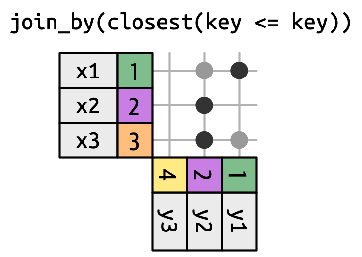
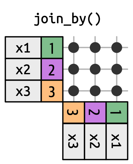
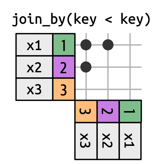
5 2 x3 y3 The joins we’ve discussed thus far have all been equi-joins, where the rows match if the x key equals the y key. But you can also specify other types of relationships.
dplyr has four different types of non-equi joins:
The joins we’ve discussed thus far have all been equi-joins, where the rows match if the x key equals the y key. But you can also specify other types of relationships.
dplyr has four different types of non-equi joins:
The joins we’ve discussed thus far have all been equi-joins, where the rows match if the x key equals the y key. But you can also specify other types of relationships.
dplyr has four different types of non-equi joins:
